【深蓝学院】移动机器人运动规划--第3章 基于采样的路径规划--作业

0. Assignment

T1. MATLAB实现RRT

1.1 GPT-4任务分析

RRT伪代码：

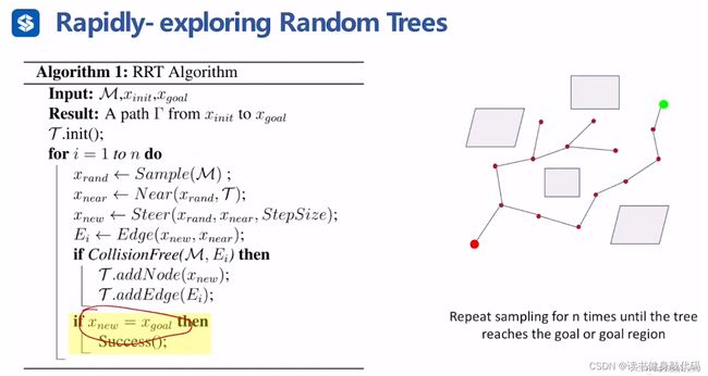
任务1即使用matlab实现RRT，结合作业所给框架，简单梳理，可结合1.2代码理解：

1. 设置start，goal，near to goal threshold Thr，step的步长Delta
2. Tree初始化，数据结构：2D xy坐标，父节点xy坐标，父节点到该节点距离，父节点的index
3. 建树部分需要我们完成：
   1. step1完成伪代码的Sample，得到x_rand
   2. step2完成伪代码的Near，具体操作：遍历树中所有Nodes，计算每个Nodes到x_rand的欧氏距离dst，取最小的，记录dst值和index
   3. step3完成伪代码的Steer，结合collisionChecking.m中进行collision checking的方法，计算方向并更新x_new
   4. step 4: 将x_new插入树T，对应伪代码Edge，CollisionFree，collision check直接调用函数，不赘述。
   5. step 5: 检查是否到达目标点附近，计算欧氏距离与Thr比较。
   6. step 6：绘图，不赘述。
4. 反向查询并绘图：
   找到goal之后，从goal回溯到父节点为start的节点，依次坐标记录到path中，最后调用MATLAB的end关键字插入一个新的node，即start，并记录start坐标，所以path中按照index顺序实际上是存储的inverse path。

   %已经遍历完path中除了起点外的所有node，end+1表示新增一个元素，所以后面再调用end时就是访问添加后的最后一个元素了
   path.pos(end+1).x = x_I; 
   path.pos(end).y = y_I;
   

   找到的path绘图为蓝色，结束。

1.2 代码

RRT.m代码：

% RRT算法
%% 流程初始化
clc
clear all; close all;
x_I=1; y_I=1;           % 设置初始点
x_G=799; y_G=799;       % 设置目标点（可尝试修改终点）
Thr=50;                 % 设置目标点阈值，用法：若当前节点和终点的欧式距离小于Thr，则跳出当前for循环
Delta= 30;              % 设置扩展步长  应该是stepsize
%% 建树初始化
T.v(1).x = x_I;         % T是我们要做的树，v是节点，这里先把起始点加入到T里面来
T.v(1).y = y_I; 
T.v(1).xPrev = x_I;     % 起始节点的父节点仍然是其本身
T.v(1).yPrev = y_I;
T.v(1).dist=0;          % 从父节点到该节点的距离，这里可取欧氏距离
T.v(1).indPrev = 0;     % 这个变量什么意思？根据下面代码来看，indPrev表示indexPrev，父节点的index
%% 开始构建树，作业部分
figure(1);
ImpRgb=imread('generate_RRT.png');
Imp=rgb2gray(ImpRgb);  %地图，255为白色，free部分
imshow(Imp)
xL=size(Imp,2);%地图x轴长度 列数
yL=size(Imp,1);%地图y轴长度 行数
hold on
plot(x_I, y_I, 'ro', 'MarkerSize',10, 'MarkerFaceColor','r');
plot(x_G, y_G, 'go', 'MarkerSize',10, 'MarkerFaceColor','g');% 绘制起点和目标点
count=1;%记录树T中节点的个数
bFind = false;

for iter = 1:3000
    x_rand=[];
    %Step 1: 在地图中随机采样一个点x_rand
    %提示：用（x_rand(1),x_rand(2)）表示环境中采样点的坐标
    x_rand(1) = rand * (xL-1) +1;%-1是为了保证随机生成的坐标不会超出地图的边界,+1是因为索引是从1开始的
    x_rand(2) = rand * (yL-1) +1;

    x_near=[];
    %Step 2: 遍历树，从树中找到最近邻近点x_near（计算每个节点到 x_rand 的距离，找出最近的一个节点作为 x_near。）
    %提示：x_near已经在树T里
    numNodes = length(T.v);
    nearest_dst = Inf;
    nearest_idx = 1;
    for node_idx = 1:numNodes
        tmp_dist = sqrt(sum(([T.v(node_idx).x T.v(node_idx).y]-[x_rand(1) x_rand(2)]).^2));%T中每个节点到x_rand的欧氏距离
        if tmp_dist < nearest_dst
            nearest_dst = tmp_dist;
            nearest_idx = node_idx;
        end
    end
    x_near(1) = T.v(nearest_idx).x;
    x_near(2) = T.v(nearest_idx).y;


    %Step 3: 扩展得到x_new节点
    %提示：注意使用扩展步长Delta
    dir=atan2(x_rand(1)-x_near(1),x_rand(2)-x_near(2));
    x_new = x_near + Delta.*[sin(dir) cos(dir)];

    
    %检查节点是否是collision-free（即是否feasiable），如果不collision-free，则继续下一次采样
    if ~collisionChecking(x_near,x_new,Imp) 
       continue;
    end
    count=count+1;
    
    %Step 4: 将x_new插入树T 
    %提示：新节点x_new的父节点是x_near
    T.v(count).x = x_new(1);
    T.v(count).y = x_new(2);
    T.v(count).xPrev = x_I;
    T.v(count).yPrev = y_I;
    T.v(count).dist = nearest_dst;
    T.v(count).indPrev = nearest_idx;

    
    %Step 5:检查是否到达目标点附近 
    %提示：注意使用目标点阈值Thr，若当前节点和终点的欧式距离小于Thr，则跳出当前for循环（退出前需要绘制出x_near和x_new之间的路径）
    check_dist = calDist(x_new, [x_G y_G]);
    if check_dist < Thr
    plot([x_near(1); x_new(1);], [x_near(2); x_new(2)], 'r', 'Linewidth', 3);
        hold on;
        bFind = true;
        break;
    end
    
    %Step 6:将x_near和x_new之间的路径画出来
    %提示 1：使用plot绘制，因为要多次在同一张图上绘制线段，所以每次使用plot后需要接上hold on命令
    %提示 2：在判断终点条件弹出for循环前，记得把x_near和x_new之间的路径画出来
    plot([x_near(1); x_new(1);], [x_near(2); x_new(2)], 'r', 'Linewidth', 3);

    pause(0.05); %暂停一会，使得RRT扩展过程容易观察
end

if T.v(count).x == T.v(end).x && T.v(count).y == T.v(end).y
    fprintf('T.v(count) == T.v(end), T.v(count): (%f, %f),  T.v(end): (%f, %f)\n', T.v(count).x, T.v(count).y,T.v(end).x, T.v(end).y);
else
    fprintf('T.v(count) != T.v(end)\n');
end

%% 路径已经找到，反向查询
if bFind
    path.pos(1).x = x_G; path.pos(1).y = y_G;
    path.pos(2).x = T.v(end).x; path.pos(2).y = T.v(end).y;%关键字end用于表示
    pathIndex = T.v(end).indPrev; % 终点加入路径
    j=0;
    while 1
        path.pos(j+3).x = T.v(pathIndex).x;
        path.pos(j+3).y = T.v(pathIndex).y;
        pathIndex = T.v(pathIndex).indPrev;
        if pathIndex == 1
            break
        end
        j=j+1;
    end  % 沿终点回溯到起点
    % 起点加入路径
    path.pos(end+1).x = x_I; %已经遍历完path中除了起点外的所有node，end+1表示新增一个元素，所以后面再调用end时就是访问添加后的最后一个元素了，没毛病
    path.pos(end).y = y_I;
    for j = 2:length(path.pos)
        plot([path.pos(j).x; path.pos(j-1).x;], [path.pos(j).y; path.pos(j-1).y], 'b', 'Linewidth', 3);
    end
else
    disp('Error, no path found!');
end

calDist.m代码：

function dist=calDist(startPose,goalPose)
dist=sqrt(sum((startPose-goalPose).^2));

1.3实验结果

如下所示：

1.4 更改Map

根据其中加载的数据，我们可以使用OpenCV生成其他类型的地图，下面是代码，在createRRTMap可以简单更改障碍物形状，上面实验使用的是我自己生成的map。

#include 
#include 
#include
using namespace cv;
using namespace std;

#include 
#include 
using namespace cv;

void createRRTMap(Mat &mat)
{
    mat = cv::Mat(mat.rows, mat.cols, CV_8UC1, cv::Scalar(255)).clone();
    for(int i = 100; i < 200; ++i)
        for(int j = 100; j < 200; ++j)
            mat.at<uint8_t>(i, j) = 0;

    for(int i = 400; i < 700; ++i)
        for(int j = 300; j < 600; ++j)
            mat.at<uint8_t>(i, j) = 0;

    for(int i = 100; i < 300; ++i)
        for(int j = 270; j < 700; ++j)
            mat.at<uint8_t>(i, j) = 0;
}

int main( )
{
    Mat matRRT(800, 800, CV_8UC1);
    Mat matRRT_rgb(800, 800, CV_8UC1);
    createRRTMap(matRRT);
    cv::cvtColor(matRRT, matRRT_rgb, cv::COLOR_GRAY2BGR);

	vector<int>compression_params;
    compression_params.push_back(CV_IMWRITE_JPEG_QUALITY);//对于PNG格式的图片，表示压缩级别，值为[0, 9]，值越大，尺寸越小，压缩时间越长
    compression_params.push_back(95);

	//显示图片
	try{
        imwrite("generate_RRT.png", matRRT_rgb, compression_params);
        imshow("生成的RRT png图",matRRT_rgb);
        fprintf(stdout,"PNG图片文件的alpha数据保存完毕~\n可以在工程目录下查看由imwrite函数生成的图片\n");
        waitKey(0);
	}
	catch(runtime_error& ex) {
		fprintf(stderr,"图像转换成PNG格式发生错误：%s\n", ex.what());
		return 1;
	}
	return 0;
}

T2. C++实现RRT*

2.1 关于K-D树的介绍

K-D树（K-Dimensional Tree的简称）是一种用于组织k维空间中的点的数据结构。这种数据结构方便了对多维空间的快速搜索，经常被用于各种数据库和计算机视觉中的快速检索任务。

K-D树是一棵二叉树，其中每个节点都是k维数值点。构造K-D树时，数据会递归地被划分成两个半空间，这个过程类似于二分查找算法。构建树的一个典型方法是选择一个维度，并在这个维度上找到位于中间的值作为划分点，将数据集分为两个子集，然后在子集上重复这个过程，但每次选择不同的维度，直到满足某个终止条件（如每个节点下的点的数量小于一定阈值）。

在K-D树的每个节点上，选择的维度和该维度上的值定义了一个超平面，这个超平面将空间分成两半，每半空间对应树中的一个分支。

搜索时，如果要找的点在划分平面的一边，就进入对应的子树继续搜索。这样可以忽略掉空间中的一大半区域，从而快速缩小搜索范围。不过需要注意的是，最近邻搜索时可能需要检查两边的子树，因为最近的点可能在划分平面的另一侧。

K-D树的优势是在处理多维数据点时提供了比线性搜索更快的查询时间，尤其是在数据点数量很大时。然而，当维数增加时，K-D树的效率会下降，这种现象被称为“维度的诅咒”。在这种情况下，可能需要考虑其他类型的数据结构，如球树或近似最近邻方法。

总结：K-D树是一颗二叉树，其中每个节点都是k维数值点，便于高维查找，当使用最近邻搜索时可能需要检查两边的子树，因为最近的点可能在划分平面的另一侧。维数增加会导致查找效率下降。

2.2 kd_nearest3 执行K-D树最近邻搜索

1. kd_nearest_i()具体搜索

   1. 搜索过程，分割不会减小搜索空间维度。
      步骤：整个空间，分割空间，子区域，左/右子树的(超)矩形

   2. 近边界（nearer boundary）和远边界（farther boundary）的更新
      

   3. K-D树搜索结束条件，效率高，大数据量搜索效率提升明显，随着维度升高，效率下降。
      
      

static void kd_nearest_i(struct kdnode *node, const double *pos, struct kdnode **result, double *result_dist_sq, struct kdhyperrect *rect)
{
    int dir = node->dir;//在第几维上分割搜索空间
    int i;
    double dummy, dist_sq;
    struct kdnode *nearer_subtree, *farther_subtree;
    double *nearer_hyperrect_coord, *farther_hyperrect_coord;//近边界和远边界

    /* Decide whether to go left or right in the tree */
    dummy = pos[dir] - node->pos[dir];
    if (dummy <= 0)  //pos <= node, pos放node左边
    {
        nearer_subtree = node->left;
        farther_subtree = node->right;
        //在第dir维上更新划分依据：rect->max离node更近，rect->min离node更远，这是指针操作，不是数值加法，
        //指针指向了新的划分边界,近边界是rect的第dir维max，远边界是dir维min
        nearer_hyperrect_coord = rect->max + dir;
        farther_hyperrect_coord = rect->min + dir;
    }
    else
    {
        nearer_subtree = node->right;
        farther_subtree = node->left;
        nearer_hyperrect_coord = rect->min + dir;
        farther_hyperrect_coord = rect->max + dir;
    }

    if (nearer_subtree)
    {
        /* Slice the hyperrect to get the hyperrect of the nearer subtree */  //递归时其实已经改变了rect的值
        dummy = *nearer_hyperrect_coord;//备份
        *nearer_hyperrect_coord = node->pos[dir];//更新rect的judge的维度的值，下一次递归使用这新维度的值来进行judge，新维度上该值为本次root节点上该维度的值(相当于本次用过了这个维度)
        /* Recurse down into nearer subtree */
        kd_nearest_i(nearer_subtree, pos, result, result_dist_sq, rect);
        /* Undo the slice */
        *nearer_hyperrect_coord = dummy;
    }

    /* Check the distance of the point at the current node, compare it
     * with our best so far */
    dist_sq = 0;
    for (i = 0; i < rect->dim; i++)
    {
        dist_sq += SQ(node->pos[i] - pos[i]);
    }
    if (dist_sq < *result_dist_sq)
    {
        *result = node;
        *result_dist_sq = dist_sq;
    }

    if (farther_subtree)
    {
        /* Get the hyperrect of the farther subtree */
        dummy = *farther_hyperrect_coord;
        *farther_hyperrect_coord = node->pos[dir];
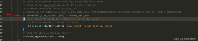
        /* Check if we have to recurse down by calculating the closest
         * point of the hyperrect and see if it's closer than our
         * minimum distance in result_dist_sq. */
        //在遍历完near子树，计算完result_dist_sq之后，计算farther子树上是否需要继续遍历(farther的dist是否比现有最小的dist小，如果小，则需要继续搜)
        if (hyperrect_dist_sq(rect, pos) < *result_dist_sq)
        {
            /* Recurse down into farther subtree */
            kd_nearest_i(farther_subtree, pos, result, result_dist_sq, rect);
        }
        /* Undo the slice on the hyperrect */
        *farther_hyperrect_coord = dummy;
    }
}

2. 搜索结束后rlist_insert插入result node，插入之后，list->next指向的是itemd所指的kdnode
3. kd_res_rewind使得rset指向result的knode。
4. void* 类型安全转换为RRTNode3DPtr类型，即TreeNode*类型。

2.3 chooseParent部分实现

该部分作业中的代码和ZJU-FAST-LAB中的代码有所区别，后者主要考虑其他算法的兼容性，在数据结构上有所不同，而作业主要针对RRT*，所以数据结构更简单。

理解了K-D tree的数据结构以及RRT* 的改进点之后，实现该部分代码比较容易，这里使用了std::multimap，先计算所有range内的edge dist并插入std::multimap中，会自动按key升序排序，然后从前到后进行collision checking，找到第一个collision-free的就找到了Parent。

 // TODO Choose a parent according to potential cost-from-start values
 // ! Hints:
 // !  1. Use map_ptr_->isSegmentValid(p1, p2) to check line edge validity;
 // !  2. Default parent is [nearest_node];
 // !  3. Store your chosen parent-node-pointer, the according cost-from-parent and cost-from-start
 // !     in [min_node], [cost_from_p], and [min_dist_from_start], respectively;
 // !  4. [Optional] You can sort the potential parents first in increasing order by cost-from-start value;
 // !  5. [Optional] You can store the collison-checking results for later usage in the Rewire procedure.
 // ! Implement your own code inside the following loop
 if(use_chooseParent_) {
     std::multimap<double, std::pair<RRTNode3DPtr, double>> mmp_neighbor_nodes;
     for (auto &curr_node : neighbour_nodes)
     {
         double dist2curr_node = calDist(curr_node->x, x_new);
         double dist_from_start = curr_node->cost_from_start + dist2curr_node;//不同前驱的更新的cost-to-come
         double tmp_cost_from_p = dist2curr_node;//cost-from-parent，即edge_cost
         mmp_neighbor_nodes.insert(std::make_pair(dist_from_start, std::make_pair(curr_node, tmp_cost_from_p)));
     }
     int mmp_count = 0;
     for(auto &each_item : mmp_neighbor_nodes) {
         ++mmp_count;
         if(map_ptr_->isSegmentValid(x_new, each_item.second.first->x)) {
             min_dist_from_start = each_item.first;
             cost_from_p = each_item.second.second;
             min_node = each_item.second.first;
             ROS_DEBUG("\nmmp_count: %d, neighbor size: %lu, collision-free, \tcur_dist_from_start: %.10f, cur_cost_from_p: %.10f",
                       mmp_count, neighbour_nodes.size(), each_item.first, each_item.second.second);
             break;
         } else {
             ROS_DEBUG("\nmmp_count: %d, neighbor size: %lu, collisioned, continue, \tcur_dist_from_start: %.10f, cur_cost_from_p: %.10f",
                       mmp_count, neighbour_nodes.size(), each_item.first, each_item.second.second);
         }
     }
 }
 // ! Implement your own code inside the above loop

2.4 Rewire

该部分代码如下：

 /* 3.rewire */
 // TODO Rewire according to potential cost-from-start values
 // ! Hints:
 // !  1. Use map_ptr_->isSegmentValid(p1, p2) to check line edge validity;
 // !  2. Use changeNodeParent(node, parent, cost_from_parent) to change a node's parent;
 // !  3. the variable [new_node] is the pointer of X_new;
 // !  4. [Optional] You can test whether the node is promising before checking edge collison.
 // ! Implement your own code between the dash lines [--------------] in the following loop
 //如果没有rewire，这里的RRT*其实和RRT没有太大区别，唯一的区别就是选取parent时使用K-D树选取了最近邻的node，
 //而RRT遍历所有现有node，直接选取距离sampling node欧氏距离最近的node作为parent
 if(use_rewire_) {
     for (auto &curr_node : neighbour_nodes)
     {
       double best_cost_before_rewire = goal_node_->cost_from_start;
       // ! -------------------------------------
       double cost_new_node_to_neighbor = calDist(new_node->x, curr_node->x);
       bool is_connected2neighbor = map_ptr_->isSegmentValid(new_node->x, goal_node_->x);
       bool is_better_path = curr_node->cost_from_start > cost_new_node_to_neighbor + new_node->cost_from_start;
       if(is_connected2neighbor && is_better_path) {
           changeNodeParent(curr_node, new_node, cost_new_node_to_neighbor);
         }
       // ! -------------------------------------
       //找到更优的解之后进行更新
       if (best_cost_before_rewire > goal_node_->cost_from_start)
       {
         vector<Eigen::Vector3d> curr_best_path;
         fillPath(goal_node_, curr_best_path);
         path_list_.emplace_back(curr_best_path);
         solution_cost_time_pair_list_.emplace_back(goal_node_->cost_from_start, (ros::Time::now() - rrt_start_time).toSec());
       }
     }
 }
 /* end of rewire */

涉及到changeNodeParent()更改节点A的父节点，以及节点A的子节点的cost_from_start值。
因为改了节点A的父节点，则节点A的子节点的cost_from_start都会改变，需要更新，使用队列，层序遍历，changeNodeParent少量注释：

void changeNodeParent(RRTNode3DPtr &node, RRTNode3DPtr &parent, const double &cost_from_parent)
{
  //更改node A的parent，首先需要删掉node A与之前parent的edge，再添加新的edge，这里的操作就是remove旧node
  if (node->parent)
    node->parent->children.remove(node); //DON'T FORGET THIS, remove it form its parent's children list（因为是改变了前驱节点，所以之前的前驱节点要删掉）
  node->parent = parent;
  node->cost_from_parent = cost_from_parent;
  node->cost_from_start = parent->cost_from_start + cost_from_parent;
  parent->children.push_back(node);

  // for all its descedants, change the cost_from_start and tau_from_start;  改了节点A的父节点，则节点A的子节点的cost_from_start都会改变，需要更新，使用队列，层序遍历
  RRTNode3DPtr descendant(node);
  std::queue<RRTNode3DPtr> Q;
  Q.push(descendant);
  while (!Q.empty())
  {
    descendant = Q.front();
    Q.pop();
    for (const auto &leafptr : descendant->children)
    {
      leafptr->cost_from_start = leafptr->cost_from_parent + descendant->cost_from_start;//主要是descendant->cost_from_start变了
      Q.push(leafptr);
    }
  }
}

2.5 对比实验

进行以下两组对比实验：

1. 相同地图和start，不同goal时，RRT*有无rewire的对比
2. 相同地图和start，不同goal时，RRT于RRT* 的对比（使用ZJU-FAST-LAB实验室的公开工作完成，其中RRT与RRT* 数据结构均为K-D tree）

2.5.1 实验1

由于RRT* 相较于RRT的改进主要在chooseParent和Rewire，而其中Rewire起主要作用，因为如果没有rewire，RRT*与RRT区别不大，所以实验1基于课程所给代码，通过是否添加Rewire来对比Rewire的优化效果。

fix地图和start(-15.4994, -20.669, 0.4)，由于ramdom sampling存在随机性，所以针对每个fixed goal，每种算法跑5次，最终取均值，共选取4个不同位置的goal，如下图所示

1. goal1：16.0521, 20.033, 0.64

RRT* without Rewire

组号	first path time cost(ms)	first path len	final path len
1	0.00186324	56.4169	54.0687
2	0.00213942	71.3945	55.3649
3	0.00082703	60.82	54.9993
4	0.000634712	56.5303	55.5882
5	0.000444331	63.243	54.713
avg	0.005908733	61.68094	54.94682

RRT* with Rewire

组号	first path time cost(ms)	first path len	final path len
1	0.00129776	58.2626	53.4338
2	0.00220048	60.8224	53.6165
3	0.000686174	54.2649	52.3802
4	0.000682761	59.3242	53.2708
5	0.000867198	58.2678	52.2388
avg	0.0011468	58.188	52.988

goal1 RRT* with Rewire 与 RRT* without Rewire对比，first path time cost无明显差别，有Rewire操作时，final path len更优。

2. goal2：2.6292, -16.682, 0.82

RRT* without Rewire

组号	first path time cost(ms)	first path len	final path len
1	0.000153107	20.2612	19.0458
2	0.000514853	20.7946	18.892
3	0.00013657	23.8047	19.7088
4	0.00010811	20.138	19.326
5	0.000312741	19.6928	19.1867
avg	0.000245	20.9383	19.2319

RRT* Rewire

组号	first path time cost(ms)	first path len	final path len
1	0.00254839	21.3555	19.0077
2	0.0015859	62.134	18.8554
3	0.000816326	52.7366	18.9015
4	5.5032e-05	24.2389	18.9784
5	0.000101631	19.7808	19.0004
avg	0.0010	36.0492	18.9487

goal2 RRT* with Rewire时first path time cost稍长，说明在这项相关性不强，仍然是with Rewire时final path更优。

3. goal3：16.0176, -20.1551, 0.32

RRT* without Rewire

组号	first path time cost(ms)	first path len	final path len
1	0.00659001	42.741	32.7316
2	0.00263363	53.1167	35.0014
3	0.000998615	44.2444	33.8431
4	0.000316079	55.4378	33.43
5	0.000968875	37.1436	34.6206
avg	0.0023	46.5367	33.9253

RRT* with Rewire

组号	first path time cost(ms)	first path len	final path len
1	0.0143187	56.0554	32.9007
2	0.00205175	43.534	33.8006
3	0.0043136	40.4332	33.0486
4	0.000946076	41.5242	33.6446
5	0.000371171	45.0295	32.6621
avg	0.0044	45.3153	33.2113

goal3 with Rewire时path len更优。

4. goal4：-12.3907 10.2501 1.74

RRT* without Rewire

组号	first path time cost(ms)	first path len	final path len
1	0.000236902	52.8212	33.3467
2	0.000526351	48.6854	35.6416
3	0.000134126	42.5125	34.8541
4	0.00014271	45.0459	33.6717
5	9.3826e-05	35.1948	33.7898
avg	0.0002	44.8520	34.2608

RRT* with Rewire

组号	first path time cost(ms)	first path len	final path len
1	0.00728627	49.9614	34.5846
2	0.000678839	41.107	34.659
3	0.00379936	39.8739	34.0933
4	0.0010686	41.0364	34.6245
5	0.000338409	41.3941	32.8667
avg	0.0026	42.6746	34.1656

goal3 with Rewire时path len更优。

整体结论：RRT* with Rewire时final patn len会更优(更短)，对于fitst path time cost影响不大。即Rewire有效地提升了feasiable path的optimality。

2.5.2 实验2

其中还跑了RRT#，BRRT，BRRT*，后两种由于没有深入了解方法，就不在此介绍，下面根据实验结果得出初步结论。

结果：

组号	goal	Method	first path use time(ms)	first path len	final path len
1	-19.5762, -13.4801, 0.82	RRT	0.000299479	32.9703	32.9703
1	-19.5762, -13.4801, 0.82	RRT*	0.000322904	33.5886	23.9271
1	-19.5762, -13.4801, 0.82	RRT#	13.205173	9.106062	23.8874
2	16.4704, 18.2802, 1.56	RRT	0.000192407	63.1801	63.1801
2	16.4704, 18.2802, 1.56	RRT*	0.000640923	56.572	49.0807
2	16.4704, 18.2802, 1.56	RRT#	0.0013824	67.88	48.8112
3	12.1996, -14.5833, 0.6	RRT	0.00103743	49.0251	49.0251
3	12.1996, -14.5833, 0.6	RRT*	0.00132163	37.7142	33.2019
3	12.1996, -14.5833, 0.6	RRT#	0.000330199	40.8708	33.1705

结论

1. RRT找到1条feasiable solution之后就不再进行优化，由于数据结构与RRT* 类似，所以找到first path时间与RRT相近，但RRT* first path通常比RRT更优。
2. final path cost，RRT* 优于RRT，说明RRT* 的find parent和rewire对path起到了优化的作用。

T3 待做

ZJU-FAST-LAB代码中有Informed sampling和GuILD sampling的实现，都属于Informed RRT*，这个后面有时间再做。

本章完。