OpenCV学习笔记 | 边缘检测Canny算法复现 | Python
摘要
OpenCV中的边缘检测是指在图像中检测出明显的边缘轮廓线,可以通过计算图像中每个像素的梯度来实现。Canny算法是一种常用的边缘检测算法,它主要通过连续的操作来寻找边缘,包括对图像去噪、计算图像梯度、非极大值抑制和双阈值处理等步骤。
一、图片加载及添加椒盐噪声
二、中值滤波和高斯滤波去噪
三、计算每个像素点的梯度强度和方向
四、非极大值抑制算法减少非边缘
五、双阈值法确定强边缘
六 、完整代码及结果展示
初始图像
噪声图像
中值滤波去噪后的图像
梯度强度边缘检测图像
非极大值抑制算法边缘检测图像
双阈值法边缘检测图像
双阈值法离散点曲线拟合边缘检测图像
一、图片加载及添加椒盐噪声
为方便算法实现,本文仅对灰度图像进行测试。首先导入必要的库后对图片进行加载,转化成灰度图像后重置图片大小,以便最后图像输出。
import cv2 as cv
import numpy as np
import matplotlib.pyplot as plt
from scipy.interpolate import splprep, splev
from scipy import signal

image = cv.imread('D:\pythonProject2\canny_image.jpg')
image = cv.cvtColor(image, cv.COLOR_BGR2GRAY)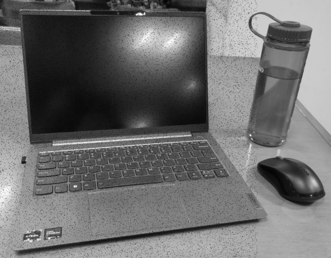
image = cv.resize(image, (928, 723))为对比不同滤波算法对图片去噪处理的能力,首先添加像素比例为0.03的椒盐噪声。椒盐噪声是数字图像处理中常见的一种噪声类型,它通常是由于传感器故障、传输过程中的干扰以及存储介质的损坏等因素引起的。它的特点是将图像中的某些像素点替换为黑色或白色,从而形成亮点或暗点,看起来就像粒子的分布一样,因此也称为“椒盐粒子噪声”。原始图片和添加了椒盐噪声的图片如图1和图2所示。
 图1 原始图片
添加椒盐噪声的函数如下:
def add_salt_and_pepper_noise(image, ratio): # 椒盐噪声
    noisy = np.copy(image)

    num_salt = int(ratio * np.size(image)) # 计算需要添加的椒盐像素个数:
    coords_row = np.random.randint(0, image.shape[0] - 1, size=num_salt)
    coords_col = np.random.randint(0, image.shape[0] - 1, size=num_salt)
    # 首先生成0到image.shape[0] - 1的随机整数,一共生成num_salt个随机数,即num_salt个椒盐噪声位置
    # 设置最大值为image.shape[0] - 1是因为索引从0开始,不能包含image.shape[0]
    coords = np.vstack((coords_row,coords_col))
    # 用vstack将椒盐噪声的行坐标列坐标组合成一个二维数组
    noisy[tuple(coords)] = 0 # 在原始图像上将coords的位置像素点变为黑色
    # 用tuple进行操作,是因为tuple是一种不可改变的数据类型,能保证添加椒盐噪声后原始图像不会改变

    return noisy
图2 添加了椒盐噪声的图片
二、中值滤波和高斯滤波去噪
中值滤波是一种常见的数字图像处理技术,用于去除数字图像中的椒盐噪声等,中值滤波不仅能去除椒盐噪声,而且能够保留图像的边缘信息。
首先设置一个3×3的核,我们将遍历整个图片的像素,将核中心的像素值替换为周围领域八个像素的中值,需要注意的是得注意核的半径,避免出现遍历到图片大小以外的位置。再一个是像素的数值都是处于0到255之间,因此在初始化时定义了np.uint8的数据类型,可以有效地降低图像数据的存储空间,节省内存,并提高计算速度。中值滤波的实现代码如下,效果如图3所示。
def median_filter(image, kernel_size): # 中值滤波
row, col = image.shape # 图像的行高和列宽
kernel_radius = kernel_size // 2 # 计算 kernel 的半径
median_image = np.zeros((row, col), np.uint8) # 初始化输出图像
# 遍历每个像素点,进行中值滤波
for y in range(kernel_radius, row - kernel_radius): # range左闭右开
for x in range(kernel_radius, col - kernel_radius):
kernel = image[y - kernel_radius:y + kernel_radius + 1, x - kernel_radius:x + kernel_radius + 1]
# 获取 kernel 区域内的像素值
median_image[y, x] = np.median(kernel) # 计算中位数并更新输出图像,注意坐标y,x
return median_image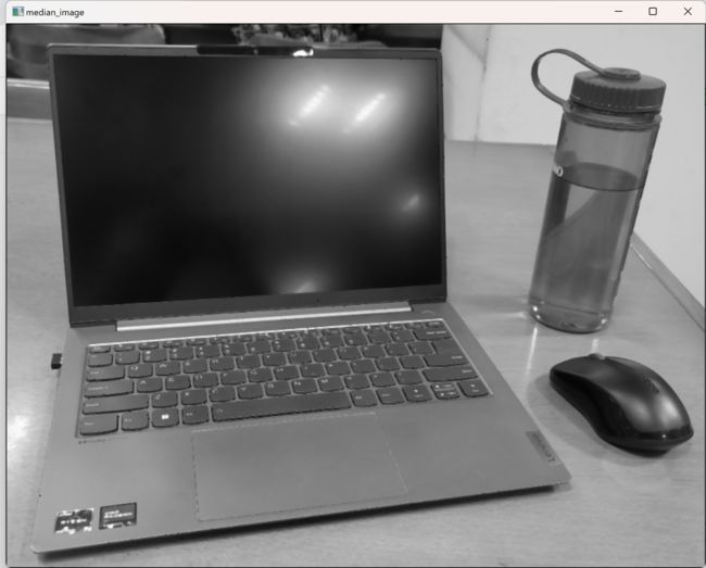 图3 中值滤波去噪后的图片
三、计算每个像素点的梯度强度和方向
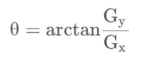
计算图像梯度强度通常使用Sobel算子,其算法基于微积分中的梯度概念,通过计算像素点周围像素值变化的差异来确定图像的边缘。假设Gx和Gy分别表示原始图像在 x 和 y 方向上的梯度,则可以使用以下Sobel算子计算梯度强度:
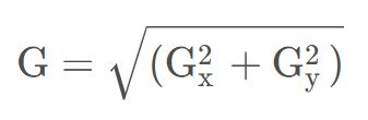 梯度强度
梯度强度
当G数值较大时,表示该点有较大的梯度强度,可以认为是图像的边缘。其中Gx和Gy的矩阵大小如下所示:
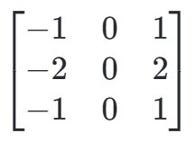 Gx
Gx 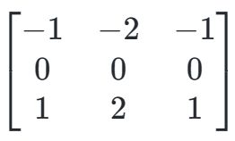 Gy
Gy
而对于梯度方向的计算,如果梯度方向在y轴上,即夹角为90°,其他情况只需代入公式计算即可,公式如下:
 梯度方向
梯度方向
实现代码如下,利用Sobel算子计算出梯度强度输出的边缘检测图片如图4所示。
def Sobel(image): # 利用Sobel算子计算每个像素点的梯度和梯度方向
# 默认窗口大小为3*3
Gx = np.array([[-1, 0, 1], [-2, 0, 2], [-1, 0, 1]])
Gy = np.array([[-1, -2, -1], [0, 0, 0], [1, 2, 1]])
row, col = image.shape
gradients = np.zeros([row - 2, col - 2])
direction = np.zeros([row - 2, col - 2])
for i in range(row - 2): # range左闭右开,从0到row-3
for j in range(col - 2): # range左闭右开,从0到col-3
dx = np.sum(image[i:i+3, j:j+3] * Gx) # 进行卷积运算
dy = np.sum(image[i:i+3, j:j+3] * Gy)
gradients[i, j] = np.sqrt(dx ** 2 + dy ** 2) # 计算每一点的梯度
if dx == 0:
direction[i, j] = np.pi / 2 # 若梯度在y轴上,那么方向夹角为90°,由于dx在分母上,因此需要单独讨论
else:
direction[i, j] = np.arctan(dy / dx) # 其余情况方向角的计算代入公式即可
gradients = np.uint8(gradients) # 由于像素的值都在0到255之间,因此需要将数值存储在8位的整型数组中
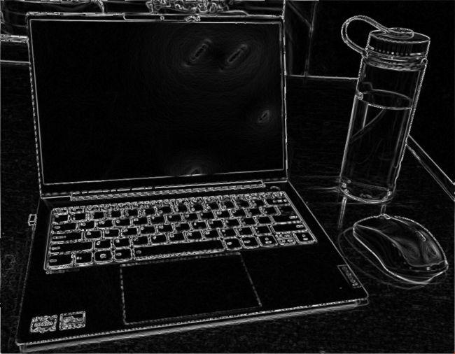
return gradients, direction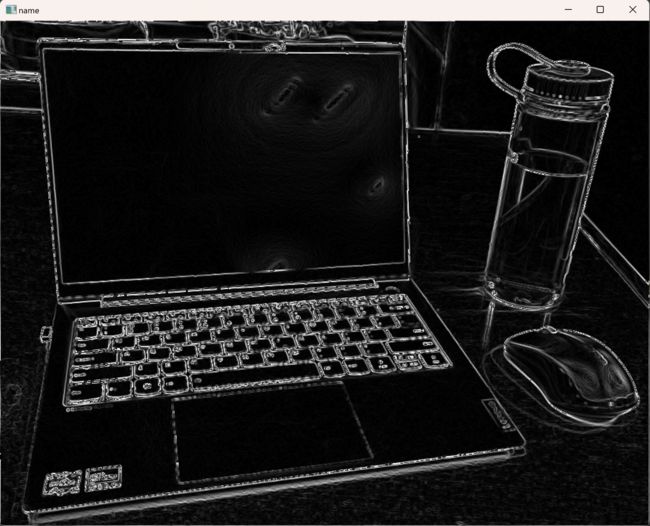 图4 梯度强度输出的边缘检测图片
四、非极大值抑制算法减少非边缘
非极大值抑制算法(Non-Maximum Suppression,NMS)是一种常见的边缘检测后处理方法,它的目的是减少由离散化边缘检测算法产生的假阳性结果(即对图像中非边缘位置赋值为边缘),从而得到更加准确的图像边缘。
首先先将Sobel算子所计算出来的梯度方向离散成水平方向(0°、180°)和对角线方向(45°、135°)以及垂直方向(90°、270°)三种类别。
-
对于水平方向,我们检查当前像素点的左右两个像素点是否比当前像素点的梯度幅值小,如果是,说明当前像素点不是一条边缘上的点之一,舍弃这个点;否则,将该像素点保留下来。
-
对于垂直方向,我们检查当前像素点的上下两个像素点是否比当前像素点的梯度幅值小,如果是,说明当前像素点不是一条边缘上的点之一,舍弃这个点;否则,将该像素点保留下来。
-
对于对角线方向,我们检查当前像素点的两个对角线方向的像素点是否比当前像素点的梯度幅值小,如果是,说明当前像素点不是一条边缘上的点之一,舍弃这个点;否则,将该像素点保留下来。
对于离散类别的角度范围如下表所示,为方便讨论,所有负数角都将加 ,转化成正数角考虑。实现代码如下,使用非极大值抑制算法检测的边缘图像如图5所示。
def non_maximum_suppression(magnitude, orientation): # 非极大值抑制算法
# magnitude:梯度强度矩阵 orientation:梯度方向矩阵
row, col = magnitude.shape # 获取尺寸信息
out_edges = np.zeros_like(magnitude) # 初始化输出矩阵
# 每个像素和周围像素点进行比较
for i in range(1, row - 1): # 该算法是要比较中间像素点和周围八个像素点的数值大小,因此需要去除首行和尾行
for j in range(1, col - 1): # 去除首列和尾列
angle = orientation[i, j] # 对每个像素点的梯度方向进行比较
if angle < 0: # 将负值角度翻转到x轴上方讨论
angle += np.pi
if (angle <= np.pi/8 or angle >= 7*np.pi/8) : # 离散成0度和180度的梯度方向
if magnitude[i, j] > magnitude[i, j - 1] and magnitude[i, j] > magnitude[i, j + 1]: # 只检查左右两个像素点的数值
out_edges[i, j] = magnitude[i, j]
elif (angle > np.pi/8 and angle <= 3*np.pi/8) or (angle >= 5*np.pi/8 and angle < 7*np.pi/8): # 离散成45度和135的梯度方向
if magnitude[i, j] > magnitude[i - 1, j - 1] and magnitude[i, j] > magnitude[i + 1, j + 1]: # 只检测对角像素点的数值
out_edges[i, j] = magnitude[i, j]
elif (angle > 3*np.pi/8 and angle < 5*np.pi/8) : # 离散成90度或270度的梯度方向
if magnitude[i, j] > magnitude[i - 1, j] and magnitude[i, j] > magnitude[i + 1, j]: # 只检测上下两个像素点的数值
out_edges[i, j] = magnitude[i, j]
return out_edges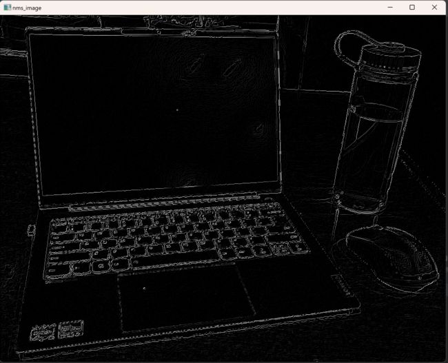 图5 非极大值边缘检测图像
五、双阈值法确定强边缘
双阈值法是Canny边缘检测算法中的一种方法,用于确定哪些边缘是真正的边缘(强边缘),哪些边缘是无关紧要的噪声(弱边缘)。
在这个算法中,我们可以通过设定低于低阈值(threshold_low)的梯度幅值的像素被认为是非边缘像素,低阈值(threshold_low)和高阈值(threshold_high)之间的像素被认为是弱边缘像素,而高于高阈值(threshold_high)的梯度幅值被认为是强边缘像素。因此该函数只需检查弱边缘像素是否与强边缘像素相连接。
对于一般的图像,可以以该阈值设置为参考去对比调整:
- threshold_low 取图像梯度幅值的平均值减一倍标准差
- threshold_high 取图像梯度幅值的平均值加一倍标准差
通常情况下,较小的最小阈值会产生更多的弱边缘,因此它可能会导致更多的总边缘数量,但同时也可能会增加边缘的错误检测率。较高的最大阈值可以消除由于噪声引起的边缘,从而可以提高边缘检测的精度,并减少误判率。但是,较高的最大阈值也可能会将实际的边缘误判为非边缘,从而导致错过一些边缘。
threshold_low 取图像梯度幅值的平均值减一倍标准差,threshold_high 取图像梯度幅值的平均值加一倍标准差,即threshold_low取-19.59,threshold_high取62.92的效果,如图6所示。
 图6 双阈值法边缘检测效果1
threshold_low取-5,threshold_high取75的效果,如图7所示。
 图7 双阈值法边缘检测效果2
threshold_low取-5,threshold_high取100的效果,如图8所示。
 图8 双阈值法边缘检测效果3
threshold_low取-5,threshold_high取85的效果,如图9所示。
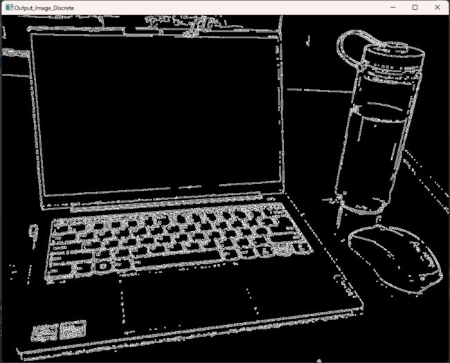 图9 双阈值法边缘检测效果4
需要注意的是,在实现算法过程中应该对图像进行拷贝,否则将会修改本地图片。代码如下。
def double_threshold_discrete(out_edges,threshold_low,threshold_high): # 双阈值法进行边缘连接
    out_pic = out_edges.copy()
    row, col = np.shape(out_pic)
    thresholded_mag = np.zeros((row, col))

    # 将满足高阈值的像素点设为强边缘像素点
    strong_i, strong_j = np.where(out_pic >= threshold_high)
    thresholded_mag[strong_i, strong_j] = 1

    # 将满足低阈值的像素点设为弱边缘像素点
    weak_i, weak_j = np.where((out_pic <= threshold_high) & (out_edges >= threshold_low))

    # 使用连通域方法连接弱边缘像素点,得到最终的边缘图像
    edge_map = np.zeros((row, col))
    for k in range(len(weak_i)):
        # 如果与确定为边缘的像素点邻接,则判定为边缘;否则为非边缘
        i = weak_i[k]
        j = weak_j[k]
        if np.any(thresholded_mag[i-1:i+2, j-1:j+2]):
            edge_map[i, j] = 1
return edge_map.astype(np.uint8)最小阈值设置为负数的时候,输出的边缘是连续性较强,而设置为正数的时候,基本上都是离散的点了,此时我们可以考虑使用splev函数进行曲线拟合。其中最小阈值设置为10,最大阈值设置为85的效果如图10所示。
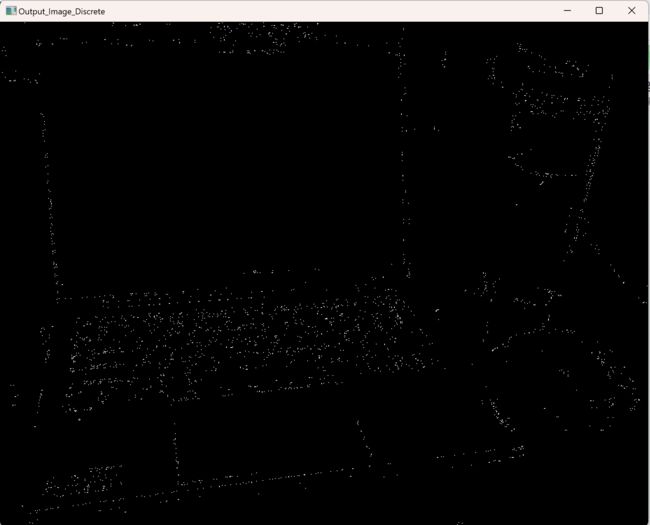 图10 双阈值法边缘检测效果5
曲线拟合实现函数如下,拟合后的效果如图11所示。由于是拟合的结果,会避免不了地出现重影模糊的情况,不推荐使用。
def double_threshold_spline(out_edges, threshold_low, threshold_high, s=500):
# 使用双阈值法进行边缘连接,得到离散的边缘点
edge_map = double_threshold_discrete(out_edges, threshold_low, threshold_high)
edge_points = np.argwhere(edge_map == 1)
# 使用样条插值进行边缘曲线拟合
tck, u = splprep(edge_points.T, s=s, per=1)
# 确定边缘曲线上的样本点
x, y = splev(u, tck)
# 将曲线上的像素点在图像上标出
out_pic = out_edges.copy()
for i in range(len(x)):
out_pic[int(x[i]), int(y[i])] = 255
return out_pic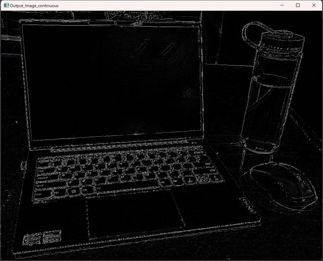 图11 双阈值法边缘检测效果6
六 、完整代码及结果展示
import cv2 as cv
import numpy as np
from scipy.interpolate import splprep, splev

def cv_show(name,image): # 图像显示
    cv.imshow('name',image)
    cv.waitKey(0)

def add_salt_and_pepper_noise(image, ratio): # 椒盐噪声
    noisy = np.copy(image)

    num_salt = int(ratio * np.size(image)) # 计算需要添加的椒盐像素个数:0.05*291600
    coords_row = np.random.randint(0, image.shape[0] - 1, size=num_salt)
    coords_col = np.random.randint(0, image.shape[0] - 1, size=num_salt)
    # 一共生成num_salt个随机数,即num_salt个椒盐噪声位置
    coords = np.vstack((coords_row,coords_col))
    # 用vstack将椒盐噪声的行坐标列坐标组合成一个二维数组
    noisy[tuple(coords)] = 0 # 在原始图像上将coords的位置像素点变为黑色
    # 用tuple进行操作,是因为tuple是一种不可改变的数据类型,能保证添加椒盐噪声后原始图像不会改变

    return noisy

def median_filter(image, kernel_size): # 中值滤波
    row, col = image.shape # 图像的行高和列宽
    kernel_radius = kernel_size // 2 # 计算 kernel 的半径

    median_image = np.zeros((row, col), np.uint8) # 初始化输出图像

    # 遍历每个像素点,进行中值滤波
    for y in range(kernel_radius, row - kernel_radius): # range左闭右开
        for x in range(kernel_radius, col - kernel_radius):
            kernel = image[y - kernel_radius:y + kernel_radius + 1, x - kernel_radius:x + kernel_radius + 1]
            # 获取 kernel 区域内的像素值
            median_image[y, x] = np.median(kernel) # 计算中位数并更新输出图像,注意坐标y,x

    return median_image

def Sobel(image): # 利用Sobel算子计算每个像素点的梯度和梯度方向
    # 默认窗口大小为3*3
    Gx = np.array([[-1, 0, 1], [-2, 0, 2], [-1, 0, 1]])
    Gy = np.array([[-1, -2, -1], [0, 0, 0], [1, 2, 1]])

    row, col = image.shape
    gradients = np.zeros([row - 2, col - 2])
    direction = np.zeros([row - 2, col - 2])

    for i in range(row - 2): # range左闭右开,从0到row-3
        for j in range(col - 2): # range左闭右开,从0到col-3
            dx = np.sum(image[i:i+3, j:j+3] * Gx) # 进行卷积运算
            dy = np.sum(image[i:i+3, j:j+3] * Gy)
            gradients[i, j] = np.sqrt(dx ** 2 + dy ** 2) # 计算每一点的梯度
            if dx == 0:
                direction[i, j] = np.pi / 2 # 若梯度在y轴上,那么方向夹角为90°,由于dx在分母上,因此需要单独讨论
            else:
                direction[i, j] = np.arctan(dy / dx) # 其余情况方向角的计算代入公式即可

    gradients = np.uint8(gradients) # 由于像素的值都在0到255之间,因此需要将数值存储在8位的整型数组中
    return gradients, direction

def non_maximum_suppression(magnitude, orientation): # 非极大值抑制算法
    # magnitude:梯度强度矩阵 orientation:梯度方向矩阵
    row, col = magnitude.shape  # 获取尺寸信息
    out_edges = np.zeros_like(magnitude)  # 初始化输出矩阵

    # 每个像素和周围像素点进行比较
    for i in range(1, row - 1): # 该算法是要比较中间像素点和周围八个像素点的数值大小,因此需要去除首行和尾行
        for j in range(1, col - 1): # 去除首列和尾列
            angle = orientation[i, j] # 对每个像素点的梯度方向进行比较
            if angle < 0: # 将负值角度翻转到x轴上方讨论
                angle += np.pi
            if (angle <= np.pi/8 or angle >= 7*np.pi/8) :  # 离散成0度和180度的梯度方向
                if magnitude[i, j] > magnitude[i, j - 1] and magnitude[i, j] > magnitude[i, j + 1]: # 只检查左右两个像素点的数值
                    out_edges[i, j] = magnitude[i, j]
            elif (angle > np.pi/8 and angle <= 3*np.pi/8) or (angle >= 5*np.pi/8 and angle < 7*np.pi/8): # 离散成45度和135的梯度方向
                if magnitude[i, j] > magnitude[i - 1, j - 1] and magnitude[i, j] > magnitude[i + 1, j + 1]: # 只检测对角像素点的数值
                    out_edges[i, j] = magnitude[i, j]
            elif (angle > 3*np.pi/8 and angle < 5*np.pi/8) : # 离散成90度或270度的梯度方向
                if magnitude[i, j] > magnitude[i - 1, j] and magnitude[i, j] > magnitude[i + 1, j]: # 只检测上下两个像素点的数值
                    out_edges[i, j] = magnitude[i, j]

    return out_edges

def double_threshold_discrete(out_edges,threshold_low,threshold_high): # 双阈值法进行边缘连接
    out_pic = out_edges.copy()
    row, col = np.shape(out_pic)
    thresholded_mag = np.zeros((row, col))

    # 将满足高阈值的像素点设为强边缘像素点
    strong_i, strong_j = np.where(out_pic >= threshold_high)
    thresholded_mag[strong_i, strong_j] = 1

    # 将满足低阈值的像素点设为弱边缘像素点
    weak_i, weak_j = np.where((out_pic <= threshold_high) & (out_edges >= threshold_low))

    # 使用连通域方法连接弱边缘像素点,得到最终的边缘图像
    edge_map = np.zeros((row, col))
    for k in range(len(weak_i)):
        # 如果与确定为边缘的像素点邻接,则判定为边缘;否则为非边缘
        i = weak_i[k]
        j = weak_j[k]
        if np.any(thresholded_mag[i-1:i+2, j-1:j+2]):
            edge_map[i, j] = 1
    return edge_map.astype(np.uint8)


def double_threshold_spline(out_edges, threshold_low, threshold_high, s=500):
    # 使用双阈值法进行边缘连接,得到离散的边缘点
    edge_map = double_threshold_discrete(out_edges, threshold_low, threshold_high)
    edge_points = np.argwhere(edge_map == 1)

    # 使用样条插值进行边缘曲线拟合
    tck, u = splprep(edge_points.T, s=s, per=1)

    # 确定边缘曲线上的样本点
    x, y = splev(u, tck)

    # 将曲线上的像素点在图像上标出
    out_pic = out_edges.copy()
    for i in range(len(x)):
        out_pic[int(x[i]), int(y[i])] = 255

    return out_pic

image = cv.imread('D:\pythonProject2\canny_image.jpg')
image = cv.cvtColor(image, cv.COLOR_BGR2GRAY)
image = cv.resize(image, (928, 723))

# 输入图片以及需要添加噪声点的比例
noisy_image = add_salt_and_pepper_noise(image,0.03)
# 中值滤波去噪
median_image = median_filter(noisy_image,3)
# 梯度强度和梯度方向
gradients,  direction = Sobel(median_image)
# 输出初始边缘检测的图像
# 统一化梯度幅值到 [0,255] 范围内
gradients_image = cv.normalize(gradients, dst=None, alpha=0, beta=255, norm_type=cv.NORM_MINMAX, dtype=cv.CV_8UC1)
# 非极大值抑制算法
nms = non_maximum_suppression(gradients,direction)
# 离散边缘检测图像
threshold_low = np.mean(gradients) - np.std(gradients)
threshold_high = np.mean(gradients) + np.std(gradients)
# print(threshold_low)
# print(threshold_high)
Output_Image_Discrete = double_threshold_discrete(nms,-5,85)
Output_Image_Discrete = Output_Image_Discrete * 255
# 使用样条插值拟合出边缘曲线
Output_Image_continuous = double_threshold_spline(nms,10,85)

cv.imshow('initial_image',image)
cv.imshow('noisy_image',noisy_image)
cv.imshow('median_image',median_image)
cv.imshow('gradients_image',gradients_image)
cv.imshow('nms_image',nms)
cv.imshow('Output_Image_Discrete',Output_Image_Discrete)
cv.imshow('Output_Image_continuous',Output_Image_continuous)
cv.waitKey(0)
cv.destroyAllWindows()
初始图像

噪声图像
中值滤波去噪后的图像

梯度强度边缘检测图像
非极大值抑制算法边缘检测图像

双阈值法边缘检测图像

双阈值法离散点曲线拟合边缘检测图像