A*搜索算法(A-Star Search)简介及保姆级代码解读

1. A*算法简单介绍

A*算法是一种路径规划算法，和传统的Dijkstra算法有所不同，该算法有选择地进行节点搜索，因此比Dijkstra算法更快、搜索的点更少。
阅读本文，不需要掌握Dijkstra算法的知识，请放心食用。
注意：本文只介绍二维A*算法及相关示例。

PS：本文代码编写参考B站up主
小黎的Ally的路径规划与轨迹跟踪系列算法学习_第4讲_A*算法，讲解详细，本文代码部分是将其代码进行了些许改动并加以解释，在此对up主的辛苦表达感谢！！

PPS：本文所使用的把地图栅格化的函数来自于博客
Matlab中将一幅图片做成栅格地图，本文进行了些许改动，再次一并感谢博主的辛苦！

1.1 A*算法理论基础

A*算法首先将要搜索的区域划分为若干栅格（grid），并有选择地标识出障碍物（Obstacle）与空白区域。一般地，栅格划分越细密，搜索点数越多，搜索过程越慢，计算量也越大；栅格划分越稀疏，搜索点数越少，相应地搜索精确性就越低。

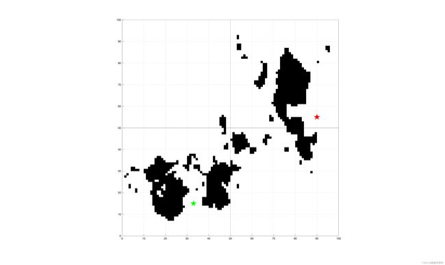
如上图，引入地图信息后画出栅格，该图片采用$100\times 100$的栅格划分，图中黑色区域为障碍物区域。图中绿点为起始点，红点为终点。

对每个节点，在计算时同时考虑两项代价指标：当前节点与起始点的距离，以及当前节点与目标点的距离：
$$f=g+h$$其中$f$为总代价，$g$为当前节点距离起始点的距离，$h$为当前节点距离目标点的距离。
而在计算距离时，又可以采用两种方式：
欧氏距离：
$$L=\sqrt{{\left(x_1-x_2\right)}^2+{\left(y_1-y_2\right)}^2}$$曼哈顿距离：
$$L=|x_1-x_2|+|y_1-y_2|$$为了计算方便，本文计算$h$时采用曼哈顿距离，这也是A*算法中的一贯做法。
为了方便计数，在计算每一个节点时，在栅格左上角写$f$值，左下角写$g$值，右下角写$h$值。

1.1.1 节点计算

这里举一个例子。

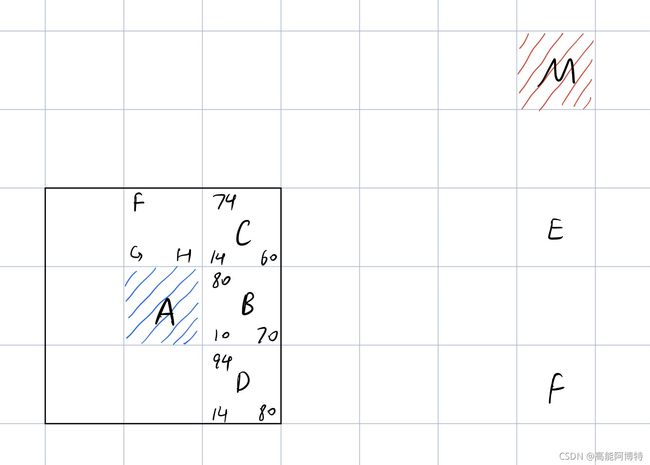
如图所示，A点为起始点，M点为终点。对于A点来说，对其周边的8个节点进行寻找，A点本身为父节点，周边8个点为子节点。

假设：

• 格子边长为10，这样水平和竖直位移一格为10，而对角位移一格为14；
• 从父节点到子节点可以水平、竖直、对角线位移计算$g$值，而从子节点到目标点只能使用水平、竖直位移计算曼哈顿距离$h$值。

对于点B：从A到B只需右移一格，因此B的$g=10$；从B到M需要先右移四格，再上移三格，因此B的$h=40+30=70$。这样B的$f=g+h=10+70=80$。将三者都记在B格中。
对于点C：从A到C只需向右上方平移一格，因此C的$g=14$；从C到M需要先右移四格，再上移两格，因此C的$h=40+20=60$，继而C的$f=g+h=74$。
同理可以计算出D的$g=14,h=80,f=94$，以及其他几个子节点的值。

将这8个子节点进行对比，可以发现，C点的$f$值最小，因此选取C点为下一步搜寻的父节点，$\overline{AC}$即为路径迈出的第一步。

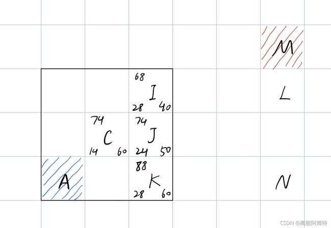
如图所示，现在将C作为新的父节点。

对于J点：
从C到J只需右移一格，因此J的$g=10+g_C=10+14=24$。需要注意的是，J点的$g$值是从C到J的$g$加上从A到C的$g$，即当前子节点的$g$值是从起点到该点的所有$g$累和。
从J到M需要先右移三格，再上移两格，因此J的$h=30+20=50$。这样J的$f=g+h=24+50=74$。将三者都记在J格中。

对于I点：
从C到I只需向右上方平移一格，同样地，I点的$g$值是从C到I的$g$加上从A到C的$g$，即当前子节点的$g$值是从起点到该点的所有$g$累和，因此I的$g=14+g_C=14+14=28$。
从I到M需要先右移三格，再上移一格，因此I的$h=30+10=40$。这样I的$f=g+h=28+40=68$。将三者都记在I格中。
同样计算出其他点的值。
可以看出，I点的$f$值最小，因此选择I点作为路径上的下一个点，此时路径变为$\overline{ACI}$。

如此一步步进行迭代，最后找到最优轨迹。

1.1.2 由计算得出的小结论

• 每个节点中需要存储至少3个值：$g,h,f$。
• 当子节点迭代到目标点本身时，$h=0$，即当前节点到目标点的距离为0.
• 在算法实施时，$g$的计算可以取10或14，即从父节点到子节点可以水平/竖直位移，也可以沿对角线位移；而$h$的计算只能取10的倍数，即从当前子节点到目标点只能水平/竖直位移。前者可以采用欧氏距离，后者只能采用曼哈顿距离。
• 当某个子节点被选中后，就作为下一次搜索的父节点；并且为了避免节点的重复计算和筛选，在下一次搜索时，需要将上一步选中的节点从“可搜索”列表中删除。如上图中，当C为父节点时，选中I作为下一次的父节点；那么当第二步I为父节点时，由于C已经在已选轨迹上了，所以I的子节点实际上并不包括C，只计算7个子节点即可。
• 鉴于上一点，可以预想，算法的具体实施过程中，需要有两个数组保存“待计算子节点”和“已被选中的节点”。当“待计算子节点”中某个点符合$f$最小时，就将其加入“已选中的节点”，并在“待计算子节点”中删除该点，防止后续重复计算。
• 当算法结束时，保存在“已选中的节点”中的所有点，按照顺序即为找出的路径。
• 算法结束时，最后一个点的$f$值，即为从起点到终点所用的距离。
• 算法的停止条件：1)当“待计算子节点”中没有点时，即已经没有点可供寻找了；2)当当前父节点恰为目标节点时，即$h=0$。

1.2 算法逻辑结构

A*算法的逻辑结构如下：
1）初始化。导入地图信息，设置障碍物区域，设置起点start、终点target、栅格数量$m\times n$等。
2）数据预处理。建立“待计算子节点”的数组openlist，“已选中的节点”的数组closelist，保存路径的数组closelist_path。除此之外，还需建立一个当前子节点集合children，用来保存当前父节点周围8个子节点的坐标，以及父节点本身parent；还有保存代价值$g,h,f$的数组openlist_cost和closelist_cost。
3）对子节点们children中的每个节点child：
若该子节点不在“待计算子节点”节点openlist中，则追加进去；
若在，则计算出该child的$g$值，该$g$值是从起点到父节点parent的距离加上父节点到该子节点的距离。若该$g$值小于之前openlist_cost中的$g$最小值，那么就将openlist_cost中的最小$g$值更新；
4）由于该代价最小点已经加入了轨迹，因此将该点加入clost_list和closelist_path，并从openlist中剔除；
5）更新openlist中的最小代价值，并以其为父节点开始新一轮搜索。

2. 代码解析

2.1 引入地图

代码块：

%% 画地图

% 栅格地图的行数、列数定义
m = 150;
n = 150;
% 地图m行n列

start = [10, 20];        % 起始节点
target = [130, 80];       % 终止节点

obs = TrunToGridMap(m, n);


% 画格子
for i = 0 : 5 : m
    plot([0, n], [i, i], 'k', 'handlevisibility', 'off');
    hold on;
end

for j = 0 : 5 : n
    plot([j, j], [0, m], 'k', 'handlevisibility', 'off');
end

axis equal;
xlim([0, n]);
ylim([0, m]);

% 绘制障碍物、起止点颜色块
scatter(start(1), start(2), 700, 'pg', 'filled');
scatter(target(1), target(2), 700, 'pr', 'filled');

for i = 1 : size(obs, 1) - 1
    temp = obs(i, :);
    fill([temp(1)-1, temp(1), temp(1), temp(1)-1],...
        [temp(2)-1, temp(2)-1, temp(2), temp(2)], 'k', 'handlevisibility', 'off');
end

temp = obs(size(obs, 1), :);
fill([temp(1)-1, temp(1), temp(1), temp(1)-1],...
    [temp(2)-1, temp(2)-1, temp(2), temp(2)], 'k');

绘制一个$150\times 150$的地图，起点设置为$(10,20)$，终点设置为$(130,80)$。
障碍物的坐标通过函数TrunToGridMap(m, n)获得：

function obs = TrunToGridMap(a, b)
    I=imread('此处放地图图片的文件名');   %读入图片
    I = rgb2gray(I);     %将图片转为灰度图
    I = imrotate(I, -90);

    l=1;    %网格边长
    B = imresize(I,[a/l b/l]);
    J=floor(B/255); 

    axes('GridLineStyle', '-');
    axis equal;

    hold on
    grid on
    axis([0,a,0,b]);
    set(gca,'xtick',0:10:a,'ytick',0:10:b);

    obs = [];

    %障碍物填充为黑色
    for i=1:a/l-1
        for j=1:b/l-1
            if(J(i,j)==0)
                obs(end+1, :) = [i, j];
            end
        end
    end
end

该函数读取一个图片文件，将其转化为灰度图像，并将灰度图中黑色色块所在的坐标返回为障碍物坐标。

2.2 预处理

%% 预处理

% 初始化closelist
closelist = start;
closelist_path = {start, start};      % 路径，从自身到自身
closelist_cost = 0;
children = child_nodes_cal(start, m, n, obs, closelist);

% 初始化openlist
openlist = children;


for i = 1 : size(openlist, 1)   % i为第i个节点
    openlist_path{i, 1} = openlist(i, :);   % openlist_path的第i行第1列为第i个节点child
    openlist_path{i, 2} = [start; openlist(i, :)]; % openlist_path的第i行第2列为一个列向量，分别是起始节点和当前child
end

for i = 1 : size(openlist, 1)
    g = norm(start - openlist(i, 1:2));
    h = abs(target(1) - openlist(i, 1)) + abs(target(2) - openlist(i, 2));
    f = g + h;
    openlist_cost(i, :) = [g, h, f];
end

这一部分主要做了以下几步：

• 把起点start设为轨迹的第一个点：closelist = start；
• 路径初始化，即从起点到起点：closelist_path = {start, start}；
• 代价首先置为0：closelist_cost = 0；
• 利用child_nodes_cal函数计算当前父节点（即起点）周围的子节点们；
• 这些子节点们children即为待计算的子节点，也就是openlist；
• 随后进入一个循环，对每一个子节点i，openlist_path中第i行第1个元素储存第i个节点child，第2个元素为一个列向量，分别是第i个child的起点和它本身；
• 第二个循环则是计算代价的循环，对每一个子节点i，计算$g$（这里使用范数norm），$h$（曼哈顿距离）和$f$；之后，在代价数组openlist_cost中储存这三个代价值，因此openlist_cost第i行的元素为一个行向量；

其中用到的子节点计算函数如下：

function child_nodes = child_nodes_cal(parent_node, m, n, obs, closelist)
    child_nodes = [];
    field = [1, 1;
        n, 1;
        n, m;
        1, m];
    
    % 左上子节点
    child_node = [parent_node(1) - 1, parent_node(2) + 1];
    if inpolygon(child_node(1), child_node(2), field(:, 1), field(:, 2))
        % [in, on] = inpolygon, 返回 in，以指明 xq 和 yq 所指定的查询点是在 xv 和 
        % yv 定义的多边形区% 域的边缘内部还是在边缘上,in为内部，on为边缘上
        if ~ismember(child_node, obs, 'rows')
            child_nodes = [child_nodes; child_node];
        end
    end
    
    
    % 上子节点
    child_node = [parent_node(1), parent_node(2) + 1];
    if inpolygon(child_node(1), child_node(2), field(:, 1), field(:, 2))
        if ~ismember(child_node, obs, 'rows')
            child_nodes = [child_nodes; child_node];
        end
    end
    
    
    % 右上子节点
    child_node = [parent_node(1) + 1, parent_node(2) + 1];
    if inpolygon(child_node(1), child_node(2), field(:, 1), field(:, 2))
        if ~ismember(child_node, obs, 'rows')
            child_nodes = [child_nodes; child_node];
        end
    end
    
    % 左子节点
    child_node = [parent_node(1) - 1, parent_node(2)];
    if inpolygon(child_node(1), child_node(2), field(:, 1), field(:, 2))
        if ~ismember(child_node, obs, 'rows')
            child_nodes = [child_nodes; child_node];
        end
    end
    
    %右子节点
    child_node = [parent_node(1) + 1, parent_node(2)];
    if inpolygon(child_node(1), child_node(2), field(:, 1), field(:, 2))
        if ~ismember(child_node, obs, 'rows')
            child_nodes = [child_nodes; child_node];
        end
    end
    
    
    %左下子节点
    child_node = [parent_node(1) - 1, parent_node(2) - 1];
    if inpolygon(child_node(1), child_node(2), field(:, 1), field(:, 2))
        if ~ismember(child_node, obs, 'rows')
            child_nodes = [child_nodes; child_node];
        end
    end
    
    
    % 下子节点
    child_node = [parent_node(1), parent_node(2) - 1];
    if inpolygon(child_node(1), child_node(2), field(:, 1), field(:, 2))
        if ~ismember(child_node, obs, 'rows')
            child_nodes = [child_nodes; child_node];
        end
    end
    
    
    % 右下子节点
    child_node = [parent_node(1) + 1, parent_node(2) - 1];
    if inpolygon(child_node(1), child_node(2), field(:, 1), field(:, 2))
        if ~ismember(child_node, obs, 'rows')
            child_nodes = [child_nodes; child_node];
        end
    end
    
    
    %% 排除已经存在于closelist的节点
    delete_idx = [];
    for i = 1 : size(child_nodes, 1)
        if ismember(child_nodes(i, :), closelist, 'rows')
            delete_idx(end+1, :) = i;
        end
    end
    
    child_nodes(delete_idx, :) = [];
end

2.3 定义父节点parent

%% 定义父节点
% 从openlist开始搜索移动代价最小的节点
[~, min_idx] = min(openlist_cost(:, 3));    % 看f值最小，min_idx为f最小的那一行
parent = openlist(min_idx, :);% 以min_idx该行的子节点child_node为新的父节点

这一步搜索openlist_cost代价数组中$f$最小的元素，记下其索引min_idx；
随后该索引对应的openlist中的元素即为“$f$值最小的待计算子节点”，作为下一步计算的父节点parent。

2.4 主循环

%% 进入循环
flag = 1;
while flag
    % 找出父节点的忽略closelist的子节点
    children = child_nodes_cal(parent ,m, n, obs, closelist);
    
    % 判断这些子节点是否在openlist中，若在，则更新；没在，则追加到openlist中
    for i = 1 : size(children, 1)
        child = children(i, :);
        [in_flag, openlist_idx] = ismember(child, openlist, 'rows');
        % in_flag表示该child_node是否在openlist中
        % openlist_idx表示该child_node在openlist中的行数
        
        g = openlist_cost(min_idx, 1) + norm(parent - child);
        % 原来的g加上新的g
        h = abs(child(1) - target(1)) + abs(child(2) - target(2));
        f = g + h;
        
        if in_flag  % 若在，则比较更新g, f
            if g < openlist_cost(openlist_idx, 1)   
                % openlist_cost(openlist_idx,1)指的是openlist_cost中idx这一行（即child_node所在的一行）的第一个坐标，即g
                openlist_cost(openlist_idx, 1) = g;
                openlist_cost(openlist_idx, 3) = f;
                openlist_path{openlist_idx, 2} = [openlist_path{min_idx, 2}; child];
                % openlist_path的第i行第2列为一个列向量，分别是起始节点和当前child，此处定义新的起始节点为openlist_path(min_idx,2)， 而openlist_path(min_idx,2)指第min_idx行所对应的 child在openlist_path中对应的路径，相当于把新的child附加到了路径上，延长了路径
            end
        else
            openlist(end+1, :) = child;
            openlist_cost(end+1, :) = [g, h, f];
            openlist_path{end+1, 1} = child;
            openlist_path{end, 2} = [openlist_path{min_idx, 2}; child];
        end
    end
    
    
    % 从openlist移除代价最小的节点到closelist
    closelist(end+1, :) = openlist(min_idx, :);
    closelist_cost(end+1, :) = openlist_cost(min_idx, 3);
    closelist_path(end+1, :) = openlist_path(min_idx, :);
    
    % 同样地，openlist中少了该节点
    openlist(min_idx, :) = [];
    openlist_cost(min_idx, :) = [];
    openlist_path(min_idx, :) = [];
    
    
    % 重新搜索：从openlist搜索移动代价最小的节点，作为新的父节点
    [~, min_idx] = min(openlist_cost(:, 3));
    parent = openlist(min_idx, :);
    
    % 判断是否搜索到终点
    if parent == target
        closelist(end+1, :) = openlist(min_idx, :);
        closelist_cost(end+1, 1) = openlist_cost(min_idx, 1);
        closelist_path(end+1, :) = openlist_path(min_idx, :);
        flag = 0;
    end

end

2.4.1

对这一部分循环来说，首先利用child_nodes_cal函数得出当前父节点parent周围的子节点们children；
对每一个子节点child，判断其是否在“待计算子节点”openlist列表中——in_flag=1表示在列表中，同时openlist_idx为该子节点在openlist中的索引号。
判断完成后，首先计算该子节点的$g,h,f$值，注意：$g$值为父节点parent的$g$加上该child子节点的$g$值。

2.4.2

计算$g,h,f$之后，再来看子节点在openlist中的情况。由于循环中查看了parent周围所有子节点的情况，所以一定会存在某个子节点的$g$比其他子节点的$g$都小。如果找到了这样的子节点，那么就更新该子节点在openlist_cost中对应位置的$g,h,f$值。

同时，还要将该子节点加入到路径openlist_path中，即这一句代码

openlist_path{openlist_idx, 2} = [openlist_path{min_idx, 2}; child];

这行代码的含义是：
openlist_idx表示当前子节点child在openlist中的索引，min_idx表示之前所有子节点中代价最小的子节点的索引。之前在预处理一节中提到，openlist_path的第i行第2列为一个列向量，分别是父节点和当前child，相当于第2列储存了路径。

而min_idx表示“代价最小的节点”，也就是父节点parent。因此这里openlist_path{min_idx, 2}表示父节点的路径。而[openlist_path{min_idx, 2}; child]则是把新的child附加到这一个列向量上，相当于把新的child附加到路径尾端，把向量长度延长了一个child，延长了路径。

这样，[openlist_path{min_idx, 2}; child]构成了一个“父节点路径-当前child”的新路径。

把这个新路径赋值给openlist_idx索引所对应的openlist_path上，即为该openlist_idx索引对应的子节点的路径。

2.4.3

另一方面，如果该child不在openlist中，那么就把该child添加到“待计算子节点”列表中，其$g,h,f$值添加到openlist_cost代价列表中，其路径[openlist_path{min_idx, 2}; child]添加到路径openlist_path中。

2.4.4

由于移动代价最小的节点已经是路径上的一点了，所以为了避免重复计算，应当把她从“待计算子节点”列表中删除，加入“已计算节点”中，即

closelist(end+1, :) = openlist(min_idx, :);
closelist_cost(end+1, :) = openlist_cost(min_idx, 3);
closelist_path(end+1, :) = openlist_path(min_idx, :);
% openlist中少了该节点
openlist(min_idx, :) = [];
openlist_cost(min_idx, :) = [];
openlist_path(min_idx, :) = [];

仔细观察不难发现，min_idx对应的正是这一步的parent节点，直到这里，我们才把它加入到“已计算节点”列表中，在之前它一直呆在openlist中。

2.4.5

父节点加入到了“已计算节点”中了，那么下一步就没有父节点了，所以需要找出新的父节点：

 [~, min_idx] = min(openlist_cost(:, 3));
parent = openlist(min_idx, :);

同时还需要判断一下，是否已经进行到了程序结束：

% 判断是否搜索到终点
if parent == target
    closelist(end+1, :) = openlist(min_idx, :);
    closelist_cost(end+1, 1) = openlist_cost(min_idx, 1);
    closelist_path(end+1, :) = openlist_path(min_idx, :);
    flag = 0;
end

需要注意，即使当当前父节点已经是目标点了，也不要忘了把这个父节点加入到“已计算节点”中，相当于把目标点添加入路径中，形成路径上最后一个点。

2.5 画图

这一步就是将结果绘制出来了：

path_opt = closelist_path{end, 2};
% closelist_path中第二列存放路径，所以path_opt存放的是路径的(x,y)值
path_opt(:, 1) = path_opt(:, 1) - 0.5;
path_opt(:, 2) = path_opt(:, 2) - 0.5;
plot(path_opt(:, 1), path_opt(:, 2), 'm', 'linewidth', 1.5);

title(['Total length of path: ' num2str(closelist_cost(end, 1))]);
legend('Start node', 'Target node', 'Obstacle', 'Path', 'location', 'northwest');
set(gca, 'fontsize', 35, 'fontname', 'times new roman');

3. 结果

这里导入稻妻地图作为路径规划的示例，该地图多为岛屿，路径复杂，障碍物分散且数量多，十分适合作为示例使用。

将其灰度化得到

把地图划分为$m\times n=150\times 150$的栅格，并设置起点为$(10,20)$，终点为$(130,80)$：

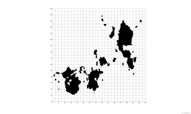
图中绿色为起点，红色为终点。

路径规划结果：

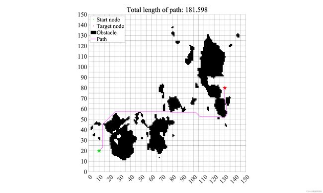
可以看出，A* 算法可以找到期望路径。

文件所有代码在笔者的资源二维A*算法路径规划matlab代码中可以下载得到。