R语言绘制热图
运用R语言绘制热图
本文主要讲述绘制热图的两种方式,分别为利用pheatmap包和ggplot2包
目录
运用R语言绘制热图
一、热图概念
二、热图绘制方法
1.利用pheatmap包
2.利用ggplot2包
一、概念
热图是一种很常见的图,其基本原则是用颜色代表数字,让数据呈现更直观、对比更明显。常用来表示不同样品组代表性基因的表达差异、不同样品组代表性化合物的含量差异、不同样品之间的两两相似性。
二、绘制方法
1.利用pheatmap包
(1)数据准备
示例如下:

(2)绘图
#加载包
> library(pheatmap)#使用pheatmap
#读取数据
> content <- read.table(file="content.txt",sep="\t",header=TRUE,
row.names=1,check.names=FALSE)
> content <- scale(content)#缩放数据
> content <- t(content)
#绘图
> pheatmap(content, cellwidth = 20, cellheight = 20,
main = "heatmap",filename = "heatmap1.png")

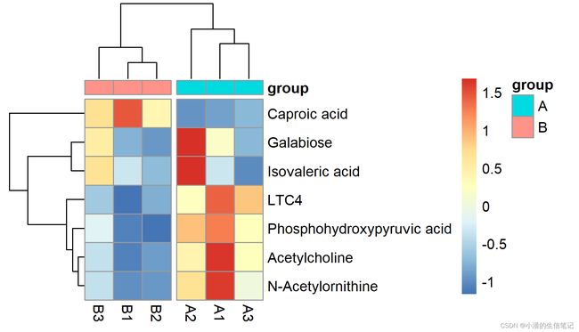
> group <-read.table(file="group.txt",sep="\t",header=TRUE,row.names=1,check.names=FALSE)
> pheatmap(content,
+          annotation_col = group,
+          cutree_cols = 2,cellwidth = 20, cellheight = 20,
+          filename = "heatmap2.png")#cutree_rows,横向切,cutree_cols,纵向切
#显示字符
> pheatmap(content1, cellwidth = 20, cellheight = 20,
display_numbers = TRUE,filename = "heatmap3.png") 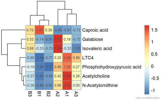
#绝对值大于1显示*号
>pheatmap(content1, cellwidth = 20, cellheight = 20,
display_numbers = matrix(ifelse(abs(content1) > 1, "*", ""),
 nrow(content1)),filename = "heatmap4.png")

2.利用ggplot2包
(1)数据准备
数据同上
(2)绘图
#加载包
> library("BiocManager")
> library("ggplot2")
> library("reshape2")
> library("ggtree")
#读取数据
> content <- read.table(file="content.txt",sep="\t",header=TRUE,row.names=1,check.names=FALSE)
> content <- scale(content)#缩放数据
> content <- t(content)
> gg <- hclust(dist(content))#对行聚类
> zz <- hclust(dist(t(content))) #对列聚类
> content <- content[gg$order,]#行,按照聚类结果排序
> data <- melt(content)#宽数据变为长数据
> data$num <- rep(c(1:7),6)#绘图时的纵坐标
> data$x <- rep(c(1:6),each = 7)#绘图时的横坐标
> ######开始绘图######
> p<-ggplot(data,aes(x=Var2,y=Var1,fill=value))+xlab("组别")+ylab("物质")
> heatmap<-p+geom_tile()+scale_fill_gradient2(low = "green", high = "red", mid = "black")
> print(heatmap)
> v <- ggtree(zz)+layout_dendrogram()# 绘制行聚类树
> #####热图和聚类树拼在一起#####
> library("aplot")
> heatmap %>% insert_top(v,height = 0.1)# 使用 aplot包里的函数进行拼图
> ggsave(file = "heatmap3.png", width = 5, height = 5,dpi=600) 