特征工程:特征提取和降维-下

目录

---

一、前言

二、正文

Ⅰ. 流形学习

Ⅱ.t-SNE

Ⅲ.多维尺度分析

三、结语

---

一、前言

 

 通过上篇对线性与非线性的数据的特征提取和降维的学习之后，我们来介绍其他方法，分别有流行学习、多维尺度分析、t-SNE。

 

二、正文

 

Ⅰ. 流形学习

 

 流形学习是借鉴拓扑流形的概念的一种降维的方法。用于数据降维，降到二维或者三维时可以对数据进行可视化。因为流形学习利用近邻的距离来计算高维空间的样本距离，所以近邻个数对其降维的结果影响甚大。

from sklearn.manifold import Isomap,MDS,TSNE
isomap=Isomap(n_neighbors=7,n_components=3)
isomap_wine_x=isomap.fit_transform(wine_x)
colors=['red','blue','green']
shape=['o','s','*']
fig=plt.figure(figsize=(10,6))
ax1=fig.add_subplot(111,projection='3d')
for ii,y in enumerate(wine_y):
      ax1.scatter(isomap_wine_x[ii,0],isomap_wine_x[ii,1],isomap_wine_x[ii,2],s=40,c=colors[y],marker=shape[y])

ax1.set_xlabel('E1',rotation=20)
ax1.set_ylabel('E2',rotation=-20)
ax1.set_zlabel('E3',rotation=90)
ax1.azim=225
ax1.set_title('Isomap')
plt.show()

 

 设置7 个近邻点来计算空间中的距离，然后n_components=3来降维到三维。

 

 

于是就能够对数据分分布情况进行可视化。 

 

Ⅱ.t-SNE

 

 t-SNE是一种常用的数据降维的方法，同时也可以作为一种数据的提取方法。

 

from sklearn.manifold import Isomap,MDS,TSNE
tsne=TSNE(n_components=3,perplexity=25,early_exaggeration=3,random_state=123)
tsne_wine_x=tsne.fit_transform(wine_x)
colors=['red','blue','green']
shape=['o','s','*']
fig=plt.figure(figsize=(10,6))
ax1=fig.add_subplot(111,projection='3d')
for ii,y in enumerate(wine_y):
      ax1.scatter(tsne_wine_x[ii,0],tsne_wine_x[ii,1],tsne_wine_x[ii,2],s=40,c=colors[y],marker=shape[y])

ax1.set_xlabel('E1',rotation=20)
ax1.set_ylabel('E2',rotation=-20)
ax1.set_zlabel('E3',rotation=90)
ax1.azim=225
ax1.set_title('Tsne')
plt.show()

 

 方法流形学习大差不大，同时提取数据上的三个特征。

 

 

 降维到三维之后开始对数据分布进行可视化。可以发现此算法下的三种数据的分布情况较容易区分，同时表明利用提取到的特征对数据类别进行分类时会更加容易。

 

Ⅲ.多维尺度分析

 

from sklearn.manifold import Isomap,MDS,TSNE
mds=MDS(n_components=3,dissimilarity='euclidean',random_state=123)
mds_wine_x=tsne.fit_transform(wine_x)
colors=['red','blue','green']
shape=['o','s','*']
fig=plt.figure(figsize=(10,6))
ax1=fig.add_subplot(111,projection='3d')
for ii,y in enumerate(wine_y):
      ax1.scatter(mds_wine_x[ii,0],mds_wine_x[ii,1],mds_wine_x[ii,2],s=40,c=colors[y],marker=shape[y])

ax1.set_xlabel('E1',rotation=20)
ax1.set_ylabel('E2',rotation=-20)
ax1.set_zlabel('E3',rotation=90)
ax1.azim=225
ax1.set_title('MDS')
plt.show()

 多维尺度分析时基于通过低维空间的可视化，从而对高维数据进行可视化的方法。其目标是：将原始数据降维到一个低维坐标系当中，同时保证通过降维引起的任何形变达到最小。

 

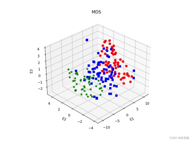
为了方便可视化该方法，通常将数据降维到二维或者三维。 

 

三、结语

 

有关特征提取和降维就到此结束，希望能够对你有所帮助，点赞收藏以备不时之需，关注我，有新的数据分析的相关文章第一时间告知你哦。