Python环境下基于最大离散重叠小波变换和支持向量回归的金融时间序列预测

金融时间序列具有非线性、高频性、随机性等特点，其波动情况不仅与当前股票市场、房地产市场、贸易市场等有强联动性，而且大幅度起伏对于其他市场有较大的影响和冲击。由于金融市场受多种因素影响且各影响因素间也存在一定复杂动态交互关系，导致金融时间序列成为一个具有非平稳性、时序相关性等特征的复杂系统，更加准确地把握金融时间序列的走势风向能够引导投资者正确的投资行为，相关的预测研究成为近几年的研究重点。因此，构建一个稳定、有效的金融时间序列预测模型是一项具有挑战性、实际应用价值的任务。

目前，金融时间序列预测方法主要可以分为计量预测方法和机器学习方法两种。一方面，计量预测方法包括差分整合移动平均自回归模型、动态模型平均、广义自回归条件异方差模型等，然而计量模型对时间序列有部分条件限制，要求时间序列的平稳性，针对非线性、非平稳数据处理效果较差。另一方面，常见的机器学习方法包括支持向量机、BP神经网络、循环神经网络等，这些模型由于在对复杂非线性、非平稳的数据进行处理时，不需要提供特定条件，具有更多的优势，获得了广泛的应用。尽管机器学习方法不是必然提升对复杂动态系统的预测准确率，但针对性的应用在非线性时间序列数据上往往能够细粒化读取数据信息、提升预测准确率。

提出一种基于最大离散重叠小波变换和支持向量回归的金融时间序列预测方法，程序运行环境为Python或Jupyter Notebook，所用模块如下：

import numpy as np
import pandas as pd
import copy
import matplotlib.pyplot as plt
from sklearn.model_selection import train_test_split
from sklearn import svm
from sklearn.metrics import mean_squared_error
from numpy.lib.stride_tricks import sliding_window_view
from modwt import modwt, modwtmra,imodwt

部分代码如下：

#第一部分，使用原始时间序列的SVM + 滑动窗口
#读取数据
prices = pd.read_csv('Data/AUD-JPY-2003-2014-day.csv',delimiter=";", header=0, encoding='utf-8', parse_dates=['Date'])
prices
# 删除不使用的列
prices.drop(["Open", "High", "Low"],axis = 1, inplace = True)
#定义变量
dates = prices['Date'].copy()
closing_prices = prices['Close'].copy()
#使用 matplotlib 绘制原始时间序列
plt.subplots(figsize=(16,4))
plt.plot(dates, closing_prices, label='Original series AUD-JPY 2003-2014')
plt.legend(loc = 'best')
plt.show()
#SVM + 滑动窗口实现
#实现滑动窗口
def slideWindow(series, window_lenght = 2):

    _X, _Y = [], []
    #Auxiliary variable to store the sliding window combinations. We sum up +1 as we are taking the last values of Aux_window
    #as the output values of our time series
    aux_Window =  sliding_window_view(series, window_lenght+1)
    #将第一个“window_lenght”值作为输入 (X)，将最后一个值 (window_lenght+1) 作为输出 (Y)
    for i in range(len(aux_Window)):
        _Y.append(aux_Window[i][-1])
        _X.append(aux_Window[i][:-1])
    
    return _X, _Y
window_lenght = 2
#调用滑动窗函数    
X, Y = slideWindow(closing_prices,window_lenght)
#25% 的数据用于测试 SVM
idx_test_date = int(0.75*len(Y)) + window_lenght
df = pd.DataFrame(columns = ['test_date']) 
df['test_date'] = prices['Date'].iloc[idx_test_date:]
##Splitting and plotting test data

#拆分和绘制测试数据，将数据拆分为训练数据（75%）和测试数据（25%） 
#shuffle = False 表示不是随机打乱数据，而是要保持有序
x_train,x_test,y_train,y_test = train_test_split(X, Y, test_size=0.25, random_state=None, shuffle=False)

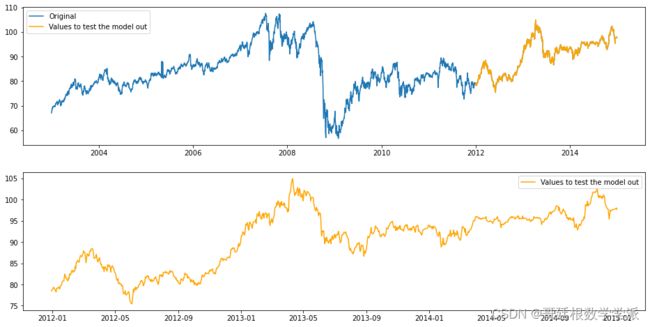
fig, ax = plt.subplots(2,1,figsize=(16,8))
ax[0].plot(dates, closing_prices, label='Original')
ax[0].plot(df['test_date'], y_test, label='Values to test the model out',color='orange')
ax[1].plot(df['test_date'], y_test, label='Values to test the model out',color='orange')

ax[0].legend(loc = 'best')
ax[1].legend(loc = 'best')
plt.show()
#构建SVR 
def evaluateSVR(_x_train,_y_train,_x_test,_y_test, kernel = 'rbf'):
    
    if (kernel == 'rbf'):
        clf = svm.SVR(kernel ='rbf', C=1e3, gamma=0.1)
    elif (kernel == 'poly'):
        clf = svm.SVR(kernel ='poly', C=1e3, degree=2)
    else:
        clf = svm.SVR(kernel ='linear',C=1e3)
    _y_predict = clf.fit(_x_train,_y_train).predict(_x_test)
    
    return _y_predict

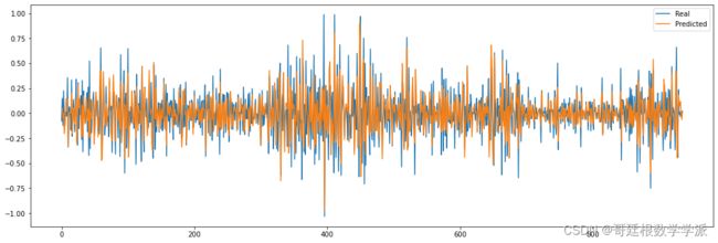
y_predict = evaluateSVR(x_train,y_train,x_test,y_test)

plotValuesWt = y_test.copy()

部分出图如下：

工学博士，担任《Mechanical System and Signal Processing》审稿专家，担任
《中国电机工程学报》优秀审稿专家，《控制与决策》，《系统工程与电子技术》，《电力系统保护与控制》，《宇航学报》等EI期刊审稿专家。

擅长领域：现代信号处理，机器学习，深度学习，数字孪生，时间序列分析，设备缺陷检测、设备异常检测、设备智能故障诊断与健康管理PHM等。