PyTorch 2.2 中文官方教程（三）

使用 PyTorch 构建模型

原文：pytorch.org/tutorials/beginner/introyt/modelsyt_tutorial.html

译者：飞龙

协议：CC BY-NC-SA 4.0

注意

点击这里下载完整示例代码

介绍 || 张量 || 自动微分 || 构建模型 || TensorBoard 支持 || 训练模型 || 模型理解

跟随下面的视频或在youtube上观看。

www.youtube.com/embed/OSqIP-mOWOI

torch.nn.Module和torch.nn.Parameter

在这个视频中，我们将讨论 PyTorch 为构建深度学习网络提供的一些工具。

除了Parameter，我们在这个视频中讨论的类都是torch.nn.Module的子类。这是 PyTorch 的基类，旨在封装特定于 PyTorch 模型及其组件的行为。

torch.nn.Module的一个重要行为是注册参数。如果特定的Module子类具有学习权重，这些权重被表示为torch.nn.Parameter的实例。Parameter类是torch.Tensor的子类，具有特殊行为，当它们被分配为Module的属性时，它们被添加到该模块的参数列表中。这些参数可以通过Module类上的parameters()方法访问。

作为一个简单的例子，这里是一个非常简单的模型，有两个线性层和一个激活函数。我们将创建一个实例，并要求它报告其参数：

import torch

class TinyModel(torch.nn.Module):

    def __init__(self):
        super(TinyModel, self).__init__()

        self.linear1 = torch.nn.Linear(100, 200)
        self.activation = torch.nn.ReLU()
        self.linear2 = torch.nn.Linear(200, 10)
        self.softmax = torch.nn.Softmax()

    def forward(self, x):
        x = self.linear1(x)
        x = self.activation(x)
        x = self.linear2(x)
        x = self.softmax(x)
        return x

tinymodel = TinyModel()

print('The model:')
print(tinymodel)

print('\n\nJust one layer:')
print(tinymodel.linear2)

print('\n\nModel params:')
for param in tinymodel.parameters():
    print(param)

print('\n\nLayer params:')
for param in tinymodel.linear2.parameters():
    print(param) 

The model:
TinyModel(
  (linear1): Linear(in_features=100, out_features=200, bias=True)
  (activation): ReLU()
  (linear2): Linear(in_features=200, out_features=10, bias=True)
  (softmax): Softmax(dim=None)
)

Just one layer:
Linear(in_features=200, out_features=10, bias=True)

Model params:
Parameter containing:
tensor([[ 0.0765,  0.0830, -0.0234,  ..., -0.0337, -0.0355, -0.0968],
        [-0.0573,  0.0250, -0.0132,  ..., -0.0060,  0.0240,  0.0280],
        [-0.0908, -0.0369,  0.0842,  ..., -0.0078, -0.0333, -0.0324],
        ...,
        [-0.0273, -0.0162, -0.0878,  ...,  0.0451,  0.0297, -0.0722],
        [ 0.0833, -0.0874, -0.0020,  ..., -0.0215,  0.0356,  0.0405],
        [-0.0637,  0.0190, -0.0571,  ..., -0.0874,  0.0176,  0.0712]],
       requires_grad=True)
Parameter containing:
tensor([ 0.0304, -0.0758, -0.0549, -0.0893, -0.0809, -0.0804, -0.0079, -0.0413,
        -0.0968,  0.0888,  0.0239, -0.0659, -0.0560, -0.0060,  0.0660, -0.0319,
        -0.0370,  0.0633, -0.0143, -0.0360,  0.0670, -0.0804,  0.0265, -0.0870,
         0.0039, -0.0174, -0.0680, -0.0531,  0.0643,  0.0794,  0.0209,  0.0419,
         0.0562, -0.0173, -0.0055,  0.0813,  0.0613, -0.0379,  0.0228,  0.0304,
        -0.0354,  0.0609, -0.0398,  0.0410,  0.0564, -0.0101, -0.0790, -0.0824,
        -0.0126,  0.0557,  0.0900,  0.0597,  0.0062, -0.0108,  0.0112, -0.0358,
        -0.0203,  0.0566, -0.0816, -0.0633, -0.0266, -0.0624, -0.0746,  0.0492,
         0.0450,  0.0530, -0.0706,  0.0308,  0.0533,  0.0202, -0.0469, -0.0448,
         0.0548,  0.0331,  0.0257, -0.0764, -0.0892,  0.0783,  0.0062,  0.0844,
        -0.0959, -0.0468, -0.0926,  0.0925,  0.0147,  0.0391,  0.0765,  0.0059,
         0.0216, -0.0724,  0.0108,  0.0701, -0.0147, -0.0693, -0.0517,  0.0029,
         0.0661,  0.0086, -0.0574,  0.0084, -0.0324,  0.0056,  0.0626, -0.0833,
        -0.0271, -0.0526,  0.0842, -0.0840, -0.0234, -0.0898, -0.0710, -0.0399,
         0.0183, -0.0883, -0.0102, -0.0545,  0.0706, -0.0646, -0.0841, -0.0095,
        -0.0823, -0.0385,  0.0327, -0.0810, -0.0404,  0.0570,  0.0740,  0.0829,
         0.0845,  0.0817, -0.0239, -0.0444, -0.0221,  0.0216,  0.0103, -0.0631,
         0.0831, -0.0273,  0.0756,  0.0022,  0.0407,  0.0072,  0.0374, -0.0608,
         0.0424, -0.0585,  0.0505, -0.0455,  0.0268, -0.0950, -0.0642,  0.0843,
         0.0760, -0.0889, -0.0617, -0.0916,  0.0102, -0.0269, -0.0011,  0.0318,
         0.0278, -0.0160,  0.0159, -0.0817,  0.0768, -0.0876, -0.0524, -0.0332,
        -0.0583,  0.0053,  0.0503, -0.0342, -0.0319, -0.0562,  0.0376, -0.0696,
         0.0735,  0.0222, -0.0775, -0.0072,  0.0294,  0.0994, -0.0355, -0.0809,
        -0.0539,  0.0245,  0.0670,  0.0032,  0.0891, -0.0694, -0.0994,  0.0126,
         0.0629,  0.0936,  0.0058, -0.0073,  0.0498,  0.0616, -0.0912, -0.0490],
       requires_grad=True)
Parameter containing:
tensor([[ 0.0504, -0.0203, -0.0573,  ...,  0.0253,  0.0642, -0.0088],
        [-0.0078, -0.0608, -0.0626,  ..., -0.0350, -0.0028, -0.0634],
        [-0.0317, -0.0202, -0.0593,  ..., -0.0280,  0.0571, -0.0114],
        ...,
        [ 0.0582, -0.0471, -0.0236,  ...,  0.0273,  0.0673,  0.0555],
        [ 0.0258, -0.0706,  0.0315,  ..., -0.0663, -0.0133,  0.0078],
        [-0.0062,  0.0544, -0.0280,  ..., -0.0303, -0.0326, -0.0462]],
       requires_grad=True)
Parameter containing:
tensor([ 0.0385, -0.0116,  0.0703,  0.0407, -0.0346, -0.0178,  0.0308, -0.0502,
         0.0616,  0.0114], requires_grad=True)

Layer params:
Parameter containing:
tensor([[ 0.0504, -0.0203, -0.0573,  ...,  0.0253,  0.0642, -0.0088],
        [-0.0078, -0.0608, -0.0626,  ..., -0.0350, -0.0028, -0.0634],
        [-0.0317, -0.0202, -0.0593,  ..., -0.0280,  0.0571, -0.0114],
        ...,
        [ 0.0582, -0.0471, -0.0236,  ...,  0.0273,  0.0673,  0.0555],
        [ 0.0258, -0.0706,  0.0315,  ..., -0.0663, -0.0133,  0.0078],
        [-0.0062,  0.0544, -0.0280,  ..., -0.0303, -0.0326, -0.0462]],
       requires_grad=True)
Parameter containing:
tensor([ 0.0385, -0.0116,  0.0703,  0.0407, -0.0346, -0.0178,  0.0308, -0.0502,
         0.0616,  0.0114], requires_grad=True) 

这显示了 PyTorch 模型的基本结构：有一个__init__()方法定义了模型的层和其他组件，还有一个forward()方法用于执行计算。注意我们可以打印模型或其子模块来了解其结构。

常见的层类型

线性层

最基本的神经网络层类型是线性或全连接层。这是一个每个输入都影响层的每个输出的程度由层的权重指定的层。如果一个模型有m个输入和n个输出，权重将是一个m x n矩阵。例如：

lin = torch.nn.Linear(3, 2)
x = torch.rand(1, 3)
print('Input:')
print(x)

print('\n\nWeight and Bias parameters:')
for param in lin.parameters():
    print(param)

y = lin(x)
print('\n\nOutput:')
print(y) 

Input:
tensor([[0.8790, 0.9774, 0.2547]])

Weight and Bias parameters:
Parameter containing:
tensor([[ 0.1656,  0.4969, -0.4972],
        [-0.2035, -0.2579, -0.3780]], requires_grad=True)
Parameter containing:
tensor([0.3768, 0.3781], requires_grad=True)

Output:
tensor([[ 0.8814, -0.1492]], grad_fn=<AddmmBackward0>) 

如果对x进行矩阵乘法，乘以线性层的权重，并加上偏置，你会发现得到输出向量y。

还有一个重要的特点需要注意：当我们用lin.weight检查层的权重时，它报告自己是一个Parameter（它是Tensor的子类），并告诉我们它正在使用 autograd 跟踪梯度。这是Parameter的默认行为，与Tensor不同。

线性层在深度学习模型中被广泛使用。你最常见到它们的地方之一是在分类器模型中，通常在末尾会有一个或多个线性层，最后一层将有n个输出，其中n是分类器处理的类的数量。

卷积层

卷积层被设计用于处理具有高度空间相关性的数据。它们在计算机视觉中非常常见，用于检测特征的紧密组合，然后将其组合成更高级的特征。它们也出现在其他上下文中 - 例如，在 NLP 应用中，一个词的即时上下文（即，序列中附近的其他词）可以影响句子的含义。

我们在早期的视频中看到了 LeNet5 中卷积层的作用：

import torch.functional as F

class LeNet(torch.nn.Module):

    def __init__(self):
        super(LeNet, self).__init__()
        # 1 input image channel (black & white), 6 output channels, 5x5 square convolution
        # kernel
        self.conv1 = torch.nn.Conv2d(1, 6, 5)
        self.conv2 = torch.nn.Conv2d(6, 16, 3)
        # an affine operation: y = Wx + b
        self.fc1 = torch.nn.Linear(16 * 6 * 6, 120)  # 6*6 from image dimension
        self.fc2 = torch.nn.Linear(120, 84)
        self.fc3 = torch.nn.Linear(84, 10)

    def forward(self, x):
        # Max pooling over a (2, 2) window
        x = F.max_pool2d(F.relu(self.conv1(x)), (2, 2))
        # If the size is a square you can only specify a single number
        x = F.max_pool2d(F.relu(self.conv2(x)), 2)
        x = x.view(-1, self.num_flat_features(x))
        x = F.relu(self.fc1(x))
        x = F.relu(self.fc2(x))
        x = self.fc3(x)
        return x

    def num_flat_features(self, x):
        size = x.size()[1:]  # all dimensions except the batch dimension
        num_features = 1
        for s in size:
            num_features *= s
        return num_features 

让我们分解一下这个模型的卷积层中发生的事情。从conv1开始：

• LeNet5 旨在接收 1x32x32 的黑白图像。**卷积层构造函数的第一个参数是输入通道的数量。**这里是 1。如果我们构建这个模型来查看 3 色通道，那么它将是 3。

• 卷积层就像一个窗口，扫描图像，寻找它认识的模式。这些模式称为特征，卷积层的一个参数是我们希望它学习的特征数量。**构造函数的第二个参数是输出特征的数量。**在这里，我们要求我们的层学习 6 个特征。

• 在上面，我将卷积层比作一个窗口 - 但窗口有多大呢？**第三个参数是窗口或内核大小。**在这里，“5”表示我们选择了一个 5x5 的内核。（如果您想要高度与宽度不同的内核，可以为此参数指定一个元组 - 例如，(3, 5)以获得一个 3x5 的卷积内核。）

卷积层的输出是一个激活图 - 表示输入张量中特征存在的空间表示。conv1将给我们一个 6x28x28 的输出张量；6 是特征的数量，28 是我们地图的高度和宽度。（28 来自于在 32 像素行上扫描 5 像素窗口时，只有 28 个有效位置的事实。）

然后我们通过 ReLU 激活函数（稍后会详细介绍激活函数）将卷积的输出传递，然后通过一个最大池化层。最大池化层将激活图中相邻的特征组合在一起。它通过减少张量，将输出中的每个 2x2 组合的单元格合并为一个单元格，并将该单元格分配为其中输入的 4 个单元格的最大值。这给我们一个激活图的低分辨率版本，尺寸为 6x14x14。

我们的下一个卷积层conv2期望 6 个输入通道（对应于第一层寻找的 6 个特征），有 16 个输出通道和一个 3x3 的内核。它输出一个 16x12x12 的激活图，然后再通过最大池化层减少到 16x6x6。在将此输出传递给线性层之前，它被重新塑造为一个 16 * 6 * 6 = 576 元素的向量，以供下一层使用。

有用于处理 1D、2D 和 3D 张量的卷积层。卷积层构造函数还有许多可选参数，包括步长（例如，仅扫描每第二个或第三个位置）在输入中，填充（这样您可以扫描到输入的边缘）等。有关更多信息，请参阅文档。

循环层

循环神经网络（或RNNs）用于顺序数据 - 从科学仪器的时间序列测量到自然语言句子到 DNA 核苷酸。RNN 通过保持作为其迄今为止在序列中看到的记忆的隐藏状态来实现这一点。

RNN 层的内部结构 - 或其变体，LSTM（长短期记忆）和 GRU（门控循环单元） - 是适度复杂的，超出了本视频的范围，但我们将通过一个基于 LSTM 的词性标注器来展示其工作原理（一种告诉你一个词是名词、动词等的分类器）：

class LSTMTagger(torch.nn.Module):

    def __init__(self, embedding_dim, hidden_dim, vocab_size, tagset_size):
        super(LSTMTagger, self).__init__()
        self.hidden_dim = hidden_dim

        self.word_embeddings = torch.nn.Embedding(vocab_size, embedding_dim)

        # The LSTM takes word embeddings as inputs, and outputs hidden states
        # with dimensionality hidden_dim.
        self.lstm = torch.nn.LSTM(embedding_dim, hidden_dim)

        # The linear layer that maps from hidden state space to tag space
        self.hidden2tag = torch.nn.Linear(hidden_dim, tagset_size)

    def forward(self, sentence):
        embeds = self.word_embeddings(sentence)
        lstm_out, _ = self.lstm(embeds.view(len(sentence), 1, -1))
        tag_space = self.hidden2tag(lstm_out.view(len(sentence), -1))
        tag_scores = F.log_softmax(tag_space, dim=1)
        return tag_scores 

构造函数有四个参数：

• vocab_size是输入词汇表中单词的数量。每个单词是一个在vocab_size维空间中的单热向量（或单位向量）。

• tagset_size是输出集合中标签的数量。

• embedding_dim是词汇表的嵌入空间的大小。嵌入将词汇表映射到一个低维空间，其中具有相似含义的单词在空间中靠在一起。

• hidden_dim是 LSTM 的记忆大小。

输入将是一个句子，其中单词表示为单热向量的索引。嵌入层将把这些映射到一个embedding_dim维空间。LSTM 接受这些嵌入的序列并对其进行迭代，生成一个长度为hidden_dim的输出向量。最终的线性层充当分类器；将log_softmax()应用于最终层的输出将输出转换为给定单词映射到给定标签的估计概率的归一化集。

如果您想看到这个网络的运行情况，请查看 pytorch.org 上的序列模型和 LSTM 网络教程。

变压器

变压器是多功能网络，已经在 NLP 领域的最新技术中占据主导地位，如 BERT 模型。变压器架构的讨论超出了本视频的范围，但 PyTorch 有一个Transformer类，允许您定义变压器模型的整体参数 - 注意头的数量，编码器和解码器层数的数量，dropout 和激活函数等（您甚至可以根据正确的参数从这个单一类构建 BERT 模型！）。torch.nn.Transformer类还有类来封装各个组件（TransformerEncoder，TransformerDecoder）和子组件（TransformerEncoderLayer，TransformerDecoderLayer）。有关详细信息，请查看 pytorch.org 上有关变压器类的文档，以及有关 pytorch.org 上相关的教程。

其他层和函数

数据操作层

还有其他层类型在模型中执行重要功能，但本身不参与学习过程。

最大池化（以及它的孪生，最小池化）通过组合单元格并将输入单元格的最大值分配给输出单元格来减少张量（我们看到了这一点）。例如：

my_tensor = torch.rand(1, 6, 6)
print(my_tensor)

maxpool_layer = torch.nn.MaxPool2d(3)
print(maxpool_layer(my_tensor)) 

tensor([[[0.5036, 0.6285, 0.3460, 0.7817, 0.9876, 0.0074],
         [0.3969, 0.7950, 0.1449, 0.4110, 0.8216, 0.6235],
         [0.2347, 0.3741, 0.4997, 0.9737, 0.1741, 0.4616],
         [0.3962, 0.9970, 0.8778, 0.4292, 0.2772, 0.9926],
         [0.4406, 0.3624, 0.8960, 0.6484, 0.5544, 0.9501],
         [0.2489, 0.8971, 0.7499, 0.1803, 0.9571, 0.6733]]])
tensor([[[0.7950, 0.9876],
         [0.9970, 0.9926]]]) 

如果您仔细查看上面的数值，您会发现 maxpooled 输出中的每个值都是 6x6 输入的每个象限的最大值。

归一化层在将一个层的输出重新居中和归一化之前将其馈送到另一个层。对中间张量进行居中和缩放具有许多有益的效果，例如让您在不爆炸/消失梯度的情况下使用更高的学习速率。

my_tensor = torch.rand(1, 4, 4) * 20 + 5
print(my_tensor)

print(my_tensor.mean())

norm_layer = torch.nn.BatchNorm1d(4)
normed_tensor = norm_layer(my_tensor)
print(normed_tensor)

print(normed_tensor.mean()) 

tensor([[[ 7.7375, 23.5649,  6.8452, 16.3517],
         [19.5792, 20.3254,  6.1930, 23.7576],
         [23.7554, 20.8565, 18.4241,  8.5742],
         [22.5100, 15.6154, 13.5698, 11.8411]]])
tensor(16.2188)
tensor([[[-0.8614,  1.4543, -0.9919,  0.3990],
         [ 0.3160,  0.4274, -1.6834,  0.9400],
         [ 1.0256,  0.5176,  0.0914, -1.6346],
         [ 1.6352, -0.0663, -0.5711, -0.9978]]],
       grad_fn=<NativeBatchNormBackward0>)
tensor(3.3528e-08, grad_fn=<MeanBackward0>) 

运行上面的单元格，我们向输入张量添加了一个大的缩放因子和偏移量；您应该看到输入张量的mean()大约在 15 的附近。通过归一化层后，您会看到值变小，并围绕零分组 - 实际上，均值应该非常小（> 1e-8）。

这是有益的，因为许多激活函数（下面讨论）在 0 附近具有最强的梯度，但有时会因为输入将它们远离零而出现消失或爆炸梯度。保持数据围绕梯度最陡峭的区域将倾向于意味着更快、更好的学习和更高的可行学习速度。

Dropout 层是鼓励模型中稀疏表示的工具 - 也就是说，推动它使用更少的数据进行推理。

Dropout 层通过在训练期间随机设置输入张量的部分来工作 - 推断时始终关闭 dropout 层。这迫使模型学习针对这个掩码或减少的数据集。例如：

my_tensor = torch.rand(1, 4, 4)

dropout = torch.nn.Dropout(p=0.4)
print(dropout(my_tensor))
print(dropout(my_tensor)) 

tensor([[[0.8869, 0.6595, 0.2098, 0.0000],
         [0.5379, 0.0000, 0.0000, 0.0000],
         [0.1950, 0.2424, 1.3319, 0.5738],
         [0.5676, 0.8335, 0.0000, 0.2928]]])
tensor([[[0.8869, 0.6595, 0.2098, 0.2878],
         [0.5379, 0.0000, 0.4029, 0.0000],
         [0.0000, 0.2424, 1.3319, 0.5738],
         [0.0000, 0.8335, 0.9647, 0.0000]]]) 

在上面，您可以看到对样本张量的 dropout 效果。您可以使用可选的p参数设置单个权重丢失的概率；如果不设置，默认为 0.5。

激活函数

激活函数使深度学习成为可能。神经网络实际上是一个程序 - 具有许多参数 - 模拟数学函数。如果我们只是重复地将张量乘以层权重，我们只能模拟线性函数；此外，拥有许多层也没有意义，因为整个网络可以简化为单个矩阵乘法。在层之间插入非线性激活函数是让深度学习模型能够模拟任何函数，而不仅仅是线性函数的关键。

torch.nn.Module 包含了封装所有主要激活函数的对象，包括 ReLU 及其许多变体，Tanh，Hardtanh，sigmoid 等。它还包括其他函数，如 Softmax，在模型的输出阶段最有用。

损失函数

损失函数告诉我们模型的预测与正确答案之间有多远。PyTorch 包含各种损失函数，包括常见的 MSE（均方误差 = L2 范数），交叉熵损失和负对数似然损失（对分类器有用），以及其他函数。

脚本的总运行时间：（0 分钟 0.029 秒）

下载 Python 源代码：modelsyt_tutorial.py

下载 Jupyter 笔记本：modelsyt_tutorial.ipynb

Sphinx-Gallery 生成的图库

PyTorch TensorBoard 支持

原文：pytorch.org/tutorials/beginner/introyt/tensorboardyt_tutorial.html

译者：飞龙

协议：CC BY-NC-SA 4.0

注意

点击这里下载完整示例代码

介绍 || 张量 || 自动微分 || 构建模型 || TensorBoard 支持 || 训练模型 || 模型理解

请跟随下面的视频或youtube。

www.youtube.com/embed/6CEld3hZgqc

开始之前

要运行此教程，您需要安装 PyTorch、TorchVision、Matplotlib 和 TensorBoard。

使用conda：

conda  install  pytorch  torchvision  -c  pytorch
conda  install  matplotlib  tensorboard 

使用pip：

pip  install  torch  torchvision  matplotlib  tensorboard 

安装完依赖项后，在安装它们的 Python 环境中重新启动此笔记本。

介绍

在本笔记本中，我们将针对时尚-MNIST 数据集训练 LeNet-5 的变体。时尚-MNIST 是一组图像瓷砖，描绘了各种服装，有十个类标签表示所描绘的服装类型。

# PyTorch model and training necessities
import torch
import torch.nn as nn
import torch.nn.functional as F
import torch.optim as optim

# Image datasets and image manipulation
import torchvision
import torchvision.transforms as transforms

# Image display
import matplotlib.pyplot as plt
import numpy as np

# PyTorch TensorBoard support
from torch.utils.tensorboard import SummaryWriter

# In case you are using an environment that has TensorFlow installed,
# such as Google Colab, uncomment the following code to avoid
# a bug with saving embeddings to your TensorBoard directory

# import tensorflow as tf
# import tensorboard as tb
# tf.io.gfile = tb.compat.tensorflow_stub.io.gfile 

在 TensorBoard 中显示图像

让我们从我们的数据集中向 TensorBoard 添加样本图像：

# Gather datasets and prepare them for consumption
transform = transforms.Compose(
    [transforms.ToTensor(),
    transforms.Normalize((0.5,), (0.5,))])

# Store separate training and validations splits in ./data
training_set = torchvision.datasets.FashionMNIST('./data',
    download=True,
    train=True,
    transform=transform)
validation_set = torchvision.datasets.FashionMNIST('./data',
    download=True,
    train=False,
    transform=transform)

training_loader = torch.utils.data.DataLoader(training_set,
                                              batch_size=4,
                                              shuffle=True,
                                              num_workers=2)

validation_loader = torch.utils.data.DataLoader(validation_set,
                                                batch_size=4,
                                                shuffle=False,
                                                num_workers=2)

# Class labels
classes = ('T-shirt/top', 'Trouser', 'Pullover', 'Dress', 'Coat',
        'Sandal', 'Shirt', 'Sneaker', 'Bag', 'Ankle Boot')

# Helper function for inline image display
def matplotlib_imshow(img, one_channel=False):
    if one_channel:
        img = img.mean(dim=0)
    img = img / 2 + 0.5     # unnormalize
    npimg = img.numpy()
    if one_channel:
        plt.imshow(npimg, cmap="Greys")
    else:
        plt.imshow(np.transpose(npimg, (1, 2, 0)))

# Extract a batch of 4 images
dataiter = iter(training_loader)
images, labels = next(dataiter)

# Create a grid from the images and show them
img_grid = torchvision.utils.make_grid(images)
matplotlib_imshow(img_grid, one_channel=True) 

Downloading http://fashion-mnist.s3-website.eu-central-1.amazonaws.com/train-images-idx3-ubyte.gz
Downloading http://fashion-mnist.s3-website.eu-central-1.amazonaws.com/train-images-idx3-ubyte.gz to ./data/FashionMNIST/raw/train-images-idx3-ubyte.gz

  0%|          | 0/26421880 [00:00<?, ?it/s]
  0%|          | 65536/26421880 [00:00<01:09, 378414.86it/s]
  1%|          | 229376/26421880 [00:00<00:37, 693250.36it/s]
  4%|3         | 950272/26421880 [00:00<00:11, 2219214.26it/s]
 15%|#4        | 3833856/26421880 [00:00<00:02, 7688687.97it/s]
 35%|###5      | 9273344/26421880 [00:00<00:01, 15802443.73it/s]
 58%|#####7    | 15204352/26421880 [00:01<00:00, 21640902.59it/s]
 80%|#######9  | 21102592/26421880 [00:01<00:00, 25246743.30it/s]
100%|##########| 26421880/26421880 [00:01<00:00, 19515987.25it/s]
Extracting ./data/FashionMNIST/raw/train-images-idx3-ubyte.gz to ./data/FashionMNIST/raw

Downloading http://fashion-mnist.s3-website.eu-central-1.amazonaws.com/train-labels-idx1-ubyte.gz
Downloading http://fashion-mnist.s3-website.eu-central-1.amazonaws.com/train-labels-idx1-ubyte.gz to ./data/FashionMNIST/raw/train-labels-idx1-ubyte.gz

  0%|          | 0/29515 [00:00<?, ?it/s]
100%|##########| 29515/29515 [00:00<00:00, 329627.44it/s]
Extracting ./data/FashionMNIST/raw/train-labels-idx1-ubyte.gz to ./data/FashionMNIST/raw

Downloading http://fashion-mnist.s3-website.eu-central-1.amazonaws.com/t10k-images-idx3-ubyte.gz
Downloading http://fashion-mnist.s3-website.eu-central-1.amazonaws.com/t10k-images-idx3-ubyte.gz to ./data/FashionMNIST/raw/t10k-images-idx3-ubyte.gz

  0%|          | 0/4422102 [00:00<?, ?it/s]
  1%|1         | 65536/4422102 [00:00<00:11, 363060.61it/s]
  5%|5         | 229376/4422102 [00:00<00:06, 683092.95it/s]
 19%|#8        | 819200/4422102 [00:00<00:01, 1861301.92it/s]
 64%|######4   | 2850816/4422102 [00:00<00:00, 5548383.23it/s]
100%|##########| 4422102/4422102 [00:00<00:00, 6080037.27it/s]
Extracting ./data/FashionMNIST/raw/t10k-images-idx3-ubyte.gz to ./data/FashionMNIST/raw

Downloading http://fashion-mnist.s3-website.eu-central-1.amazonaws.com/t10k-labels-idx1-ubyte.gz
Downloading http://fashion-mnist.s3-website.eu-central-1.amazonaws.com/t10k-labels-idx1-ubyte.gz to ./data/FashionMNIST/raw/t10k-labels-idx1-ubyte.gz

  0%|          | 0/5148 [00:00<?, ?it/s]
100%|##########| 5148/5148 [00:00<00:00, 39618856.87it/s]
Extracting ./data/FashionMNIST/raw/t10k-labels-idx1-ubyte.gz to ./data/FashionMNIST/raw 

以上，我们使用 TorchVision 和 Matplotlib 创建了一个输入数据小批量的可视网格。下面，我们使用SummaryWriter上的add_image()调用来记录图像以供 TensorBoard 使用，并调用flush()确保它立即写入磁盘。

# Default log_dir argument is "runs" - but it's good to be specific
# torch.utils.tensorboard.SummaryWriter is imported above
writer = SummaryWriter('runs/fashion_mnist_experiment_1')

# Write image data to TensorBoard log dir
writer.add_image('Four Fashion-MNIST Images', img_grid)
writer.flush()

# To view, start TensorBoard on the command line with:
#   tensorboard --logdir=runs
# ...and open a browser tab to http://localhost:6006/ 

如果您在命令行启动 TensorBoard 并在新的浏览器选项卡中打开它（通常在 localhost:6006），您应该在 IMAGES 选项卡下看到图像网格。

绘制标量以可视化训练

TensorBoard 对于跟踪训练的进展和有效性非常有用。在下面，我们将运行一个训练循环，跟踪一些指标，并保存数据供 TensorBoard 使用。

让我们定义一个模型来对我们的图像瓷砖进行分类，以及用于训练的优化器和损失函数：

class Net(nn.Module):
    def __init__(self):
        super(Net, self).__init__()
        self.conv1 = nn.Conv2d(1, 6, 5)
        self.pool = nn.MaxPool2d(2, 2)
        self.conv2 = nn.Conv2d(6, 16, 5)
        self.fc1 = nn.Linear(16 * 4 * 4, 120)
        self.fc2 = nn.Linear(120, 84)
        self.fc3 = nn.Linear(84, 10)

    def forward(self, x):
        x = self.pool(F.relu(self.conv1(x)))
        x = self.pool(F.relu(self.conv2(x)))
        x = x.view(-1, 16 * 4 * 4)
        x = F.relu(self.fc1(x))
        x = F.relu(self.fc2(x))
        x = self.fc3(x)
        return x

net = Net()
criterion = nn.CrossEntropyLoss()
optimizer = optim.SGD(net.parameters(), lr=0.001, momentum=0.9) 

现在让我们训练一个 epoch，并在每 1000 批次时评估训练与验证集的损失：

print(len(validation_loader))
for epoch in range(1):  # loop over the dataset multiple times
    running_loss = 0.0

    for i, data in enumerate(training_loader, 0):
        # basic training loop
        inputs, labels = data
        optimizer.zero_grad()
        outputs = net(inputs)
        loss = criterion(outputs, labels)
        loss.backward()
        optimizer.step()

        running_loss += loss.item()
        if i % 1000 == 999:    # Every 1000 mini-batches...
            print('Batch {}'.format(i + 1))
            # Check against the validation set
            running_vloss = 0.0

            # In evaluation mode some model specific operations can be omitted eg. dropout layer
            net.train(False) # Switching to evaluation mode, eg. turning off regularisation
            for j, vdata in enumerate(validation_loader, 0):
                vinputs, vlabels = vdata
                voutputs = net(vinputs)
                vloss = criterion(voutputs, vlabels)
                running_vloss += vloss.item()
            net.train(True) # Switching back to training mode, eg. turning on regularisation

            avg_loss = running_loss / 1000
            avg_vloss = running_vloss / len(validation_loader)

            # Log the running loss averaged per batch
            writer.add_scalars('Training vs. Validation Loss',
                            { 'Training' : avg_loss, 'Validation' : avg_vloss },
                            epoch * len(training_loader) + i)

            running_loss = 0.0
print('Finished Training')

writer.flush() 

2500
Batch 1000
Batch 2000
Batch 3000
Batch 4000
Batch 5000
Batch 6000
Batch 7000
Batch 8000
Batch 9000
Batch 10000
Batch 11000
Batch 12000
Batch 13000
Batch 14000
Batch 15000
Finished Training 

切换到您打开的 TensorBoard，并查看 SCALARS 选项卡。

可视化您的模型

TensorBoard 还可以用于检查模型内部的数据流。为此，请使用模型和样本输入调用add_graph()方法。当您打开

# Again, grab a single mini-batch of images
dataiter = iter(training_loader)
images, labels = next(dataiter)

# add_graph() will trace the sample input through your model,
# and render it as a graph.
writer.add_graph(net, images)
writer.flush() 

当您切换到 TensorBoard 时，您应该看到一个 GRAPHS 选项卡。双击“NET”节点以查看模型内部的层和数据流。

使用嵌入可视化您的数据集

我们使用的 28x28 图像瓷砖可以建模为 784 维向量（28 * 28 = 784）。将其投影到较低维度表示可能很有启发性。add_embedding()方法将一组数据投影到具有最高方差的三个维度，并将它们显示为交互式 3D 图表。add_embedding()方法通过自动投影到具有最高方差的三个维度来实现这一点。

接下来，我们将取一部分数据，并生成这样一个嵌入：

# Select a random subset of data and corresponding labels
def select_n_random(data, labels, n=100):
    assert len(data) == len(labels)

    perm = torch.randperm(len(data))
    return data[perm][:n], labels[perm][:n]

# Extract a random subset of data
images, labels = select_n_random(training_set.data, training_set.targets)

# get the class labels for each image
class_labels = [classes[label] for label in labels]

# log embeddings
features = images.view(-1, 28 * 28)
writer.add_embedding(features,
                    metadata=class_labels,
                    label_img=images.unsqueeze(1))
writer.flush()
writer.close() 

现在，如果您切换到 TensorBoard 并选择 PROJECTOR 选项卡，您应该看到投影的 3D 表示。您可以旋转和缩放模型。在大尺度和小尺度上检查它，并查看是否可以在投影数据和标签的聚类中发现模式。

为了更好地可见，建议：

• 从左侧的“按颜色分类”下拉菜单中选择“标签”。

• 在顶部切换到夜间模式图标，将浅色图像放在黑色背景上。

其他资源

有关更多信息，请查看：

• PyTorch 关于torch.utils.tensorboard.SummaryWriter的文档

• PyTorch.org 教程中的 Tensorboard 教程内容

• 有关 TensorBoard 的更多信息，请参阅TensorBoard 文档

脚本的总运行时间：（2 分钟 34.092 秒）

下载 Python 源代码：tensorboardyt_tutorial.py

下载 Jupyter 笔记本：tensorboardyt_tutorial.ipynb

Sphinx-Gallery 生成的画廊

使用 PyTorch 进行训练

原文：pytorch.org/tutorials/beginner/introyt/trainingyt.html

译者：飞龙

协议：CC BY-NC-SA 4.0

注意

点击这里下载完整示例代码

介绍 || 张量 || 自动微分 || 构建模型 || TensorBoard 支持 || 训练模型 || 模型理解

跟随下面的视频或者在youtube上进行操作。

www.youtube.com/embed/jF43_wj_DCQ

介绍

在过去的视频中，我们已经讨论并演示了：

• 使用 torch.nn 模块的神经网络层和函数构建模型

• 自动梯度计算的机制是基于梯度的模型训练的核心

• 使用 TensorBoard 来可视化训练进度和其他活动

在这个视频中，我们将为您的工具库添加一些新工具：

• 我们将熟悉数据集和数据加载器的抽象，以及它们如何简化在训练循环中向模型提供数据的过程

• 我们将讨论具体的损失函数以及何时使用它们

• 我们将研究 PyTorch 优化器，它们实现了根据损失函数的结果调整模型权重的算法。

最后，我们将把所有这些内容整合在一起，看到完整的 PyTorch 训练循环的运行。

数据集和数据加载器

Dataset和DataLoader类封装了从存储中提取数据并将其以批量形式暴露给训练循环的过程。

Dataset负责访问和处理单个数据实例。

DataLoader从Dataset中获取数据实例（自动或使用您定义的采样器），将它们收集到批次中，并返回给您的训练循环消费。DataLoader适用于所有类型的数据集，无论它们包含的数据类型是什么。

在本教程中，我们将使用 TorchVision 提供的 Fashion-MNIST 数据集。我们使用torchvision.transforms.Normalize()来将图像块内容的分布归零并进行归一化，并下载训练和验证数据拆分。

import torch
import torchvision
import torchvision.transforms as transforms

# PyTorch TensorBoard support
from torch.utils.tensorboard import SummaryWriter
from datetime import datetime

transform = transforms.Compose(
    [transforms.ToTensor(),
    transforms.Normalize((0.5,), (0.5,))])

# Create datasets for training & validation, download if necessary
training_set = torchvision.datasets.FashionMNIST('./data', train=True, transform=transform, download=True)
validation_set = torchvision.datasets.FashionMNIST('./data', train=False, transform=transform, download=True)

# Create data loaders for our datasets; shuffle for training, not for validation
training_loader = torch.utils.data.DataLoader(training_set, batch_size=4, shuffle=True)
validation_loader = torch.utils.data.DataLoader(validation_set, batch_size=4, shuffle=False)

# Class labels
classes = ('T-shirt/top', 'Trouser', 'Pullover', 'Dress', 'Coat',
        'Sandal', 'Shirt', 'Sneaker', 'Bag', 'Ankle Boot')

# Report split sizes
print('Training set has {} instances'.format(len(training_set)))
print('Validation set has {} instances'.format(len(validation_set))) 

Downloading http://fashion-mnist.s3-website.eu-central-1.amazonaws.com/train-images-idx3-ubyte.gz
Downloading http://fashion-mnist.s3-website.eu-central-1.amazonaws.com/train-images-idx3-ubyte.gz to ./data/FashionMNIST/raw/train-images-idx3-ubyte.gz

  0%|          | 0/26421880 [00:00<?, ?it/s]
  0%|          | 65536/26421880 [00:00<01:12, 364219.97it/s]
  1%|          | 229376/26421880 [00:00<00:38, 686138.70it/s]
  4%|3         | 950272/26421880 [00:00<00:11, 2201377.51it/s]
 14%|#4        | 3801088/26421880 [00:00<00:02, 7581352.34it/s]
 37%|###7      | 9797632/26421880 [00:00<00:00, 16849344.06it/s]
 59%|#####9    | 15663104/26421880 [00:01<00:00, 26145189.61it/s]
 71%|#######1  | 18776064/26421880 [00:01<00:00, 23360633.32it/s]
 93%|#########2| 24543232/26421880 [00:01<00:00, 26387177.79it/s]
100%|##########| 26421880/26421880 [00:01<00:00, 19446710.50it/s]
Extracting ./data/FashionMNIST/raw/train-images-idx3-ubyte.gz to ./data/FashionMNIST/raw

Downloading http://fashion-mnist.s3-website.eu-central-1.amazonaws.com/train-labels-idx1-ubyte.gz
Downloading http://fashion-mnist.s3-website.eu-central-1.amazonaws.com/train-labels-idx1-ubyte.gz to ./data/FashionMNIST/raw/train-labels-idx1-ubyte.gz

  0%|          | 0/29515 [00:00<?, ?it/s]
100%|##########| 29515/29515 [00:00<00:00, 326274.86it/s]
Extracting ./data/FashionMNIST/raw/train-labels-idx1-ubyte.gz to ./data/FashionMNIST/raw

Downloading http://fashion-mnist.s3-website.eu-central-1.amazonaws.com/t10k-images-idx3-ubyte.gz
Downloading http://fashion-mnist.s3-website.eu-central-1.amazonaws.com/t10k-images-idx3-ubyte.gz to ./data/FashionMNIST/raw/t10k-images-idx3-ubyte.gz

  0%|          | 0/4422102 [00:00<?, ?it/s]
  1%|1         | 65536/4422102 [00:00<00:11, 364622.91it/s]
  5%|5         | 229376/4422102 [00:00<00:06, 684813.81it/s]
 21%|##1       | 950272/4422102 [00:00<00:01, 2200476.22it/s]
 85%|########5 | 3768320/4422102 [00:00<00:00, 7506714.24it/s]
100%|##########| 4422102/4422102 [00:00<00:00, 6115026.62it/s]
Extracting ./data/FashionMNIST/raw/t10k-images-idx3-ubyte.gz to ./data/FashionMNIST/raw

Downloading http://fashion-mnist.s3-website.eu-central-1.amazonaws.com/t10k-labels-idx1-ubyte.gz
Downloading http://fashion-mnist.s3-website.eu-central-1.amazonaws.com/t10k-labels-idx1-ubyte.gz to ./data/FashionMNIST/raw/t10k-labels-idx1-ubyte.gz

  0%|          | 0/5148 [00:00<?, ?it/s]
100%|##########| 5148/5148 [00:00<00:00, 35867569.75it/s]
Extracting ./data/FashionMNIST/raw/t10k-labels-idx1-ubyte.gz to ./data/FashionMNIST/raw

Training set has 60000 instances
Validation set has 10000 instances 

像往常一样，让我们通过可视化数据来进行健全性检查：

import matplotlib.pyplot as plt
import numpy as np

# Helper function for inline image display
def matplotlib_imshow(img, one_channel=False):
    if one_channel:
        img = img.mean(dim=0)
    img = img / 2 + 0.5     # unnormalize
    npimg = img.numpy()
    if one_channel:
        plt.imshow(npimg, cmap="Greys")
    else:
        plt.imshow(np.transpose(npimg, (1, 2, 0)))

dataiter = iter(training_loader)
images, labels = next(dataiter)

# Create a grid from the images and show them
img_grid = torchvision.utils.make_grid(images)
matplotlib_imshow(img_grid, one_channel=True)
print('  '.join(classes[labels[j]] for j in range(4))) 

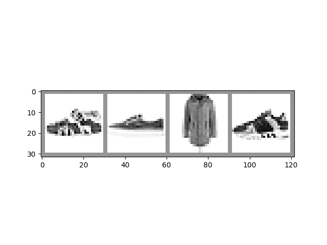
Sandal  Sneaker  Coat  Sneaker 

模型

在这个例子中，我们将使用 LeNet-5 的变体模型 - 如果您观看了本系列中的先前视频，这应该是熟悉的。

import torch.nn as nn
import torch.nn.functional as F

# PyTorch models inherit from torch.nn.Module
class GarmentClassifier(nn.Module):
    def __init__(self):
        super(GarmentClassifier, self).__init__()
        self.conv1 = nn.Conv2d(1, 6, 5)
        self.pool = nn.MaxPool2d(2, 2)
        self.conv2 = nn.Conv2d(6, 16, 5)
        self.fc1 = nn.Linear(16 * 4 * 4, 120)
        self.fc2 = nn.Linear(120, 84)
        self.fc3 = nn.Linear(84, 10)

    def forward(self, x):
        x = self.pool(F.relu(self.conv1(x)))
        x = self.pool(F.relu(self.conv2(x)))
        x = x.view(-1, 16 * 4 * 4)
        x = F.relu(self.fc1(x))
        x = F.relu(self.fc2(x))
        x = self.fc3(x)
        return x

model = GarmentClassifier() 

损失函数

在这个例子中，我们将使用交叉熵损失。为了演示目的，我们将创建一批虚拟输出和标签值，将它们通过损失函数运行，并检查结果。

loss_fn = torch.nn.CrossEntropyLoss()

# NB: Loss functions expect data in batches, so we're creating batches of 4
# Represents the model's confidence in each of the 10 classes for a given input
dummy_outputs = torch.rand(4, 10)
# Represents the correct class among the 10 being tested
dummy_labels = torch.tensor([1, 5, 3, 7])

print(dummy_outputs)
print(dummy_labels)

loss = loss_fn(dummy_outputs, dummy_labels)
print('Total loss for this batch: {}'.format(loss.item())) 

tensor([[0.7026, 0.1489, 0.0065, 0.6841, 0.4166, 0.3980, 0.9849, 0.6701, 0.4601,
         0.8599],
        [0.7461, 0.3920, 0.9978, 0.0354, 0.9843, 0.0312, 0.5989, 0.2888, 0.8170,
         0.4150],
        [0.8408, 0.5368, 0.0059, 0.8931, 0.3942, 0.7349, 0.5500, 0.0074, 0.0554,
         0.1537],
        [0.7282, 0.8755, 0.3649, 0.4566, 0.8796, 0.2390, 0.9865, 0.7549, 0.9105,
         0.5427]])
tensor([1, 5, 3, 7])
Total loss for this batch: 2.428950071334839 

优化器

在这个例子中，我们将使用带有动量的简单随机梯度下降。

尝试对这个优化方案进行一些变化可能会有帮助：

• 学习率确定了优化器采取的步长大小。不同的学习率对训练结果的准确性和收敛时间有什么影响？

• 动量在多个步骤中将优化器推向最强梯度的方向。改变这个值会对你的结果产生什么影响？

• 尝试一些不同的优化算法，比如平均 SGD、Adagrad 或 Adam。你的结果有什么不同？

# Optimizers specified in the torch.optim package
optimizer = torch.optim.SGD(model.parameters(), lr=0.001, momentum=0.9) 

训练循环

下面是一个执行一个训练周期的函数。它枚举来自 DataLoader 的数据，并在每次循环中执行以下操作：

• 从 DataLoader 获取一批训练数据

• 将优化器的梯度置零

• 执行推断 - 也就是为输入批次从模型获取预测

• 计算该批次预测与数据集标签之间的损失

• 计算学习权重的反向梯度

• 告诉优化器执行一个学习步骤 - 即根据我们选择的优化算法，根据这一批次的观察梯度调整模型的学习权重

• 它报告每 1000 批次的损失。

• 最后，它报告了最后 1000 批次的平均每批次损失，以便与验证运行进行比较

def train_one_epoch(epoch_index, tb_writer):
    running_loss = 0.
    last_loss = 0.

    # Here, we use enumerate(training_loader) instead of
    # iter(training_loader) so that we can track the batch
    # index and do some intra-epoch reporting
    for i, data in enumerate(training_loader):
        # Every data instance is an input + label pair
        inputs, labels = data

        # Zero your gradients for every batch!
        optimizer.zero_grad()

        # Make predictions for this batch
        outputs = model(inputs)

        # Compute the loss and its gradients
        loss = loss_fn(outputs, labels)
        loss.backward()

        # Adjust learning weights
        optimizer.step()

        # Gather data and report
        running_loss += loss.item()
        if i % 1000 == 999:
            last_loss = running_loss / 1000 # loss per batch
            print('  batch {} loss: {}'.format(i + 1, last_loss))
            tb_x = epoch_index * len(training_loader) + i + 1
            tb_writer.add_scalar('Loss/train', last_loss, tb_x)
            running_loss = 0.

    return last_loss 

每轮活动

每轮我们都要做一些事情：

• 通过检查在训练中未使用的一组数据上的相对损失来执行验证，并报告此结果

• 保存模型的副本

在这里，我们将在 TensorBoard 中进行报告。这将需要转到命令行启动 TensorBoard，并在另一个浏览器选项卡中打开它。

# Initializing in a separate cell so we can easily add more epochs to the same run
timestamp = datetime.now().strftime('%Y%m%d_%H%M%S')
writer = SummaryWriter('runs/fashion_trainer_{}'.format(timestamp))
epoch_number = 0

EPOCHS = 5

best_vloss = 1_000_000.

for epoch in range(EPOCHS):
    print('EPOCH {}:'.format(epoch_number + 1))

    # Make sure gradient tracking is on, and do a pass over the data
    model.train(True)
    avg_loss = train_one_epoch(epoch_number, writer)

    running_vloss = 0.0
    # Set the model to evaluation mode, disabling dropout and using population
    # statistics for batch normalization.
    model.eval()

    # Disable gradient computation and reduce memory consumption.
    with torch.no_grad():
        for i, vdata in enumerate(validation_loader):
            vinputs, vlabels = vdata
            voutputs = model(vinputs)
            vloss = loss_fn(voutputs, vlabels)
            running_vloss += vloss

    avg_vloss = running_vloss / (i + 1)
    print('LOSS train {} valid {}'.format(avg_loss, avg_vloss))

    # Log the running loss averaged per batch
    # for both training and validation
    writer.add_scalars('Training vs. Validation Loss',
                    { 'Training' : avg_loss, 'Validation' : avg_vloss },
                    epoch_number + 1)
    writer.flush()

    # Track best performance, and save the model's state
    if avg_vloss < best_vloss:
        best_vloss = avg_vloss
        model_path = 'model_{}_{}'.format(timestamp, epoch_number)
        torch.save(model.state_dict(), model_path)

    epoch_number += 1 

EPOCH 1:
  batch 1000 loss: 1.6334228584356607
  batch 2000 loss: 0.8325267538074403
  batch 3000 loss: 0.7359380583595484
  batch 4000 loss: 0.6198329215242994
  batch 5000 loss: 0.6000315657821484
  batch 6000 loss: 0.555109024874866
  batch 7000 loss: 0.5260250487388112
  batch 8000 loss: 0.4973462742221891
  batch 9000 loss: 0.4781935699362075
  batch 10000 loss: 0.47880298678041433
  batch 11000 loss: 0.45598648857555235
  batch 12000 loss: 0.4327470133750467
  batch 13000 loss: 0.41800182418141046
  batch 14000 loss: 0.4115047634313814
  batch 15000 loss: 0.4211296908891527
LOSS train 0.4211296908891527 valid 0.414460688829422
EPOCH 2:
  batch 1000 loss: 0.3879808729066281
  batch 2000 loss: 0.35912817339546743
  batch 3000 loss: 0.38074520684120944
  batch 4000 loss: 0.3614532373107213
  batch 5000 loss: 0.36850082185724753
  batch 6000 loss: 0.3703581801643886
  batch 7000 loss: 0.38547042514081115
  batch 8000 loss: 0.37846584360170527
  batch 9000 loss: 0.3341486988377292
  batch 10000 loss: 0.3433013284947956
  batch 11000 loss: 0.35607743899174965
  batch 12000 loss: 0.3499939931873523
  batch 13000 loss: 0.33874178926000603
  batch 14000 loss: 0.35130289171106416
  batch 15000 loss: 0.3394507191307202
LOSS train 0.3394507191307202 valid 0.3581162691116333
EPOCH 3:
  batch 1000 loss: 0.3319729989422485
  batch 2000 loss: 0.29558994361863006
  batch 3000 loss: 0.3107374766407593
  batch 4000 loss: 0.3298987646112146
  batch 5000 loss: 0.30858693152241906
  batch 6000 loss: 0.33916381367447684
  batch 7000 loss: 0.3105102765217889
  batch 8000 loss: 0.3011080777524912
  batch 9000 loss: 0.3142058177240979
  batch 10000 loss: 0.31458891937109
  batch 11000 loss: 0.31527258940579483
  batch 12000 loss: 0.31501667268342864
  batch 13000 loss: 0.3011875962628328
  batch 14000 loss: 0.30012811454350596
  batch 15000 loss: 0.31833117976446373
LOSS train 0.31833117976446373 valid 0.3307691514492035
EPOCH 4:
  batch 1000 loss: 0.2786161053752294
  batch 2000 loss: 0.27965198021690596
  batch 3000 loss: 0.28595415444140965
  batch 4000 loss: 0.292985666413857
  batch 5000 loss: 0.3069892351147719
  batch 6000 loss: 0.29902250939945224
  batch 7000 loss: 0.2863366014406201
  batch 8000 loss: 0.2655441066541243
  batch 9000 loss: 0.3045048695363293
  batch 10000 loss: 0.27626545656517554
  batch 11000 loss: 0.2808379335970967
  batch 12000 loss: 0.29241049340573955
  batch 13000 loss: 0.28030834131941446
  batch 14000 loss: 0.2983542350126445
  batch 15000 loss: 0.3009556676162611
LOSS train 0.3009556676162611 valid 0.41686952114105225
EPOCH 5:
  batch 1000 loss: 0.2614263167564495
  batch 2000 loss: 0.2587047562422049
  batch 3000 loss: 0.2642477260621345
  batch 4000 loss: 0.2825975873669813
  batch 5000 loss: 0.26987933717705165
  batch 6000 loss: 0.2759250026817317
  batch 7000 loss: 0.26055969463163275
  batch 8000 loss: 0.29164007206353565
  batch 9000 loss: 0.2893096504513578
  batch 10000 loss: 0.2486029507305684
  batch 11000 loss: 0.2732803234480907
  batch 12000 loss: 0.27927226484491985
  batch 13000 loss: 0.2686819267635074
  batch 14000 loss: 0.24746483912148323
  batch 15000 loss: 0.27903492261294194
LOSS train 0.27903492261294194 valid 0.31206756830215454 

加载模型的保存版本：

saved_model = GarmentClassifier()
saved_model.load_state_dict(torch.load(PATH)) 

加载模型后，它已准备好用于您需要的任何操作 - 更多训练，推断或分析。

请注意，如果您的模型具有影响模型结构的构造函数参数，您需要提供它们并将模型配置为与保存时的状态相同。

其他资源

• PyTorch 中的数据工具文档，包括 Dataset 和 DataLoader

• 关于在 GPU 训练中使用固定内存的说明

• TorchVision，TorchText和TorchAudio中可用数据集的文档

• PyTorch 中可用的损失函数的文档

• torch.optim 包的文档，其中包括优化器和相关工具，如学习率调度

• 有关保存和加载模型的详细教程

• pytorch.org 的教程部分包含广泛的训练任务教程，包括不同领域的分类，生成对抗网络，强化学习等

脚本的总运行时间：（5 分钟 4.557 秒）

下载 Python 源代码：trainingyt.py

下载 Jupyter 笔记本：trainingyt.ipynb

Sphinx-Gallery 生成的图库

使用 Captum 进行模型理解

原文：pytorch.org/tutorials/beginner/introyt/captumyt.html

译者：飞龙

协议：CC BY-NC-SA 4.0

注意

点击这里下载完整示例代码

介绍 || 张量 || 自动微分 || 构建模型 || TensorBoard 支持 || 训练模型 || 模型理解

请跟随下面的视频或YouTube进行操作。在这里下载笔记本和相应的文件这里。

www.youtube.com/embed/Am2EF9CLu-g

Captum（拉丁语中的“理解”）是一个建立在 PyTorch 上的开源、可扩展的模型可解释性库。

随着模型复杂性的增加和由此产生的不透明性，模型可解释性方法变得越来越重要。模型理解既是一个活跃的研究领域，也是一个在使用机器学习的各行业中实际应用的重点领域。Captum 提供了最先进的算法，包括集成梯度，为研究人员和开发人员提供了一种简单的方法来理解哪些特征对模型的输出有贡献。

在Captum.ai网站上提供了完整的文档、API 参考和一系列关于特定主题的教程。

介绍

Captum 对模型可解释性的方法是以归因为基础的。Captum 提供了三种类型的归因：

• 特征归因试图解释特定输出，以输入的特征生成它。例如，解释电影评论是积极的还是消极的，以评论中的某些词语为例。

• 层归因研究了模型隐藏层在特定输入后的活动。检查卷积层对输入图像的空间映射输出是层归因的一个例子。

• 神经元归因类似于层归因，但专注于单个神经元的活动。

在这个互动笔记本中，我们将查看特征归因和层归因。

每种归因类型都有多个归因算法与之相关。许多归因算法可分为两大类：

• 基于梯度的算法计算模型输出、层输出或神经元激活相对于输入的反向梯度。集成梯度（用于特征）、层梯度*激活和神经元电导都是基于梯度的算法。

• 基于扰动的算法检查模型、层或神经元对输入变化的响应。输入扰动可能是有方向的或随机的。遮挡、特征消融和特征置换都是基于扰动的算法。

我们将在下面检查这两种类型的算法。

特别是涉及大型模型时，以一种易于将其与正在检查的输入特征相关联的方式可视化归因数据可能是有价值的。虽然可以使用 Matplotlib、Plotly 或类似工具创建自己的可视化，但 Captum 提供了专门针对其归因的增强工具：

• captum.attr.visualization模块（如下导入为viz）提供了有用的函数，用于可视化与图像相关的归因。

• Captum Insights是一个易于使用的 API，位于 Captum 之上，提供了一个可视化小部件，其中包含了针对图像、文本和任意模型类型的现成可视化。

这两种可视化工具集将在本笔记本中进行演示。前几个示例将重点放在计算机视觉用例上，但最后的 Captum Insights 部分将演示在多模型、视觉问答模型中的归因可视化。

安装

在开始之前，您需要具有 Python 环境：

• Python 版本 3.6 或更高

• 对于 Captum Insights 示例，需要 Flask 1.1 或更高版本以及 Flask-Compress（建议使用最新版本）

• PyTorch 版本 1.2 或更高（建议使用最新版本）

• TorchVision 版本 0.6 或更高（建议使用最新版本）

• Captum（建议使用最新版本）

• Matplotlib 版本 3.3.4，因为 Captum 目前使用的 Matplotlib 函数在后续版本中已更名其参数

要在 Anaconda 或 pip 虚拟环境中安装 Captum，请使用下面适合您环境的命令：

使用conda：

conda  install  pytorch  torchvision  captum  flask-compress  matplotlib=3.3.4  -c  pytorch 

使用pip：

pip  install  torch  torchvision  captum  matplotlib==3.3.4  Flask-Compress 

在您设置的环境中重新启动此笔记本，然后您就可以开始了！

第一个示例

首先，让我们以一个简单的视觉示例开始。我们将使用在 ImageNet 数据集上预训练的 ResNet 模型。我们将获得一个测试输入，并使用不同的特征归因算法来检查输入图像对输出的影响，并查看一些测试图像的输入归因映射的有用可视化。

首先，一些导入：

import torch
import torch.nn.functional as F
import torchvision.transforms as transforms
import torchvision.models as models

import captum
from captum.attr import IntegratedGradients, Occlusion, LayerGradCam, LayerAttribution
from captum.attr import visualization as viz

import os, sys
import json

import numpy as np
from PIL import Image
import matplotlib.pyplot as plt
from matplotlib.colors import LinearSegmentedColormap 

现在我们将使用 TorchVision 模型库下载一个预训练的 ResNet。由于我们不是在训练，所以暂时将其置于评估模式。

model = models.resnet18(weights='IMAGENET1K_V1')
model = model.eval() 

您获取这个交互式笔记本的地方也应该有一个带有img文件夹的文件cat.jpg。

test_img = Image.open('https://gitcode.net/OpenDocCN/pytorch-doc-zh/-/raw/master/docs/2.2/img/cat.jpg')
test_img_data = np.asarray(test_img)
plt.imshow(test_img_data)
plt.show() 

我们的 ResNet 模型是在 ImageNet 数据集上训练的，并且期望图像具有特定大小，并且通道数据被归一化到特定范围的值。我们还将导入我们的模型识别的类别的可读标签列表 - 这也应该在img文件夹中。

# model expects 224x224 3-color image
transform = transforms.Compose([
 transforms.Resize(224),
 transforms.CenterCrop(224),
 transforms.ToTensor()
])

# standard ImageNet normalization
transform_normalize = transforms.Normalize(
     mean=[0.485, 0.456, 0.406],
     std=[0.229, 0.224, 0.225]
 )

transformed_img = transform(test_img)
input_img = transform_normalize(transformed_img)
input_img = input_img.unsqueeze(0) # the model requires a dummy batch dimension

labels_path = 'https://gitcode.net/OpenDocCN/pytorch-doc-zh/-/raw/master/docs/2.2/img/imagenet_class_index.json'
with open(labels_path) as json_data:
    idx_to_labels = json.load(json_data) 

现在，我们可以问一个问题：我们的模型认为这张图像代表什么？

output = model(input_img)
output = F.softmax(output, dim=1)
prediction_score, pred_label_idx = torch.topk(output, 1)
pred_label_idx.squeeze_()
predicted_label = idx_to_labels[str(pred_label_idx.item())][1]
print('Predicted:', predicted_label, '(', prediction_score.squeeze().item(), ')') 

我们已经确认 ResNet 认为我们的猫图像实际上是一只猫。但是为什么模型认为这是一张猫的图像呢？

要找到答案，我们转向 Captum。

使用集成梯度进行特征归因

特征归因将特定输出归因于输入的特征。它使用特定的输入 - 在这里，我们的测试图像 - 生成每个输入特征对特定输出特征的相对重要性的映射。

Integrated Gradients是 Captum 中可用的特征归因算法之一。集成梯度通过近似模型输出相对于输入的梯度的积分来为每个输入特征分配重要性分数。

在我们的情况下，我们将获取输出向量的特定元素 - 即指示模型对其选择的类别的信心的元素 - 并使用集成梯度来了解输入图像的哪些部分有助于此输出。

一旦我们从集成梯度获得了重要性映射，我们将使用 Captum 中的可视化工具来提供重要性映射的有用表示。Captum 的visualize_image_attr()函数提供了各种选项，用于自定义您的归因数据的显示。在这里，我们传入一个自定义的 Matplotlib 颜色映射。

运行带有integrated_gradients.attribute()调用的单元格通常需要一两分钟。

# Initialize the attribution algorithm with the model
integrated_gradients = IntegratedGradients(model)

# Ask the algorithm to attribute our output target to
attributions_ig = integrated_gradients.attribute(input_img, target=pred_label_idx, n_steps=200)

# Show the original image for comparison
_ = viz.visualize_image_attr(None, np.transpose(transformed_img.squeeze().cpu().detach().numpy(), (1,2,0)),
                      method="original_image", title="Original Image")

default_cmap = LinearSegmentedColormap.from_list('custom blue',
                                                 [(0, '#ffffff'),
                                                  (0.25, '#0000ff'),
                                                  (1, '#0000ff')], N=256)

_ = viz.visualize_image_attr(np.transpose(attributions_ig.squeeze().cpu().detach().numpy(), (1,2,0)),
                             np.transpose(transformed_img.squeeze().cpu().detach().numpy(), (1,2,0)),
                             method='heat_map',
                             cmap=default_cmap,
                             show_colorbar=True,
                             sign='positive',
                             title='Integrated Gradients') 

在上面的图像中，您应该看到集成梯度在图像中猫的位置周围给出了最强的信号。

使用遮挡进行特征归因

基于梯度的归因方法有助于理解模型，直接计算输出相对于输入的变化。基于扰动的归因方法更直接地处理这个问题，通过对输入引入变化来衡量对输出的影响。遮挡就是这样一种方法。它涉及替换输入图像的部分，并检查对输出信号的影响。

在下面，我们设置了遮挡归因。类似于配置卷积神经网络，您可以指定目标区域的大小，以及步长来确定单个测量的间距。我们将使用visualize_image_attr_multiple()来可视化我们的遮挡归因的输出，显示正面和负面归因的热图，以及通过用正面归因区域遮罩原始图像。遮罩提供了一个非常有教育意义的视图，显示了模型认为最“像猫”的猫照片的哪些区域。

occlusion = Occlusion(model)

attributions_occ = occlusion.attribute(input_img,
                                       target=pred_label_idx,
                                       strides=(3, 8, 8),
                                       sliding_window_shapes=(3,15, 15),
                                       baselines=0)

_ = viz.visualize_image_attr_multiple(np.transpose(attributions_occ.squeeze().cpu().detach().numpy(), (1,2,0)),
                                      np.transpose(transformed_img.squeeze().cpu().detach().numpy(), (1,2,0)),
                                      ["original_image", "heat_map", "heat_map", "masked_image"],
                                      ["all", "positive", "negative", "positive"],
                                      show_colorbar=True,
                                      titles=["Original", "Positive Attribution", "Negative Attribution", "Masked"],
                                      fig_size=(18, 6)
                                     ) 

同样，我们看到模型更加重视包含猫的图像区域。

使用 Layer GradCAM 的层归因

层归因允许您将模型中隐藏层的活动归因于输入的特征。在下面，我们将使用一个层归因算法来检查模型中一个卷积层的活动。

GradCAM 计算目标输出相对于给定层的梯度，对每个输出通道（输出的第 2 维）进行平均，并将每个通道的平均梯度乘以层激活。结果在所有通道上求和。GradCAM 设计用于卷积网络；由于卷积层的活动通常在空间上映射到输入，GradCAM 归因通常会被上采样并用于遮罩输入。

层归因的设置与输入归因类似，只是除了模型之外，您还必须指定要检查的模型内的隐藏层。与上面一样，当我们调用attribute()时，我们指定感兴趣的目标类。

layer_gradcam = LayerGradCam(model, model.layer3[1].conv2)
attributions_lgc = layer_gradcam.attribute(input_img, target=pred_label_idx)

_ = viz.visualize_image_attr(attributions_lgc[0].cpu().permute(1,2,0).detach().numpy(),
                             sign="all",
                             title="Layer 3 Block 1 Conv 2") 

我们将使用方便的方法interpolate()在LayerAttribution基类中，将这些归因数据上采样，以便与输入图像进行比较。

upsamp_attr_lgc = LayerAttribution.interpolate(attributions_lgc, input_img.shape[2:])

print(attributions_lgc.shape)
print(upsamp_attr_lgc.shape)
print(input_img.shape)

_ = viz.visualize_image_attr_multiple(upsamp_attr_lgc[0].cpu().permute(1,2,0).detach().numpy(),
                                      transformed_img.permute(1,2,0).numpy(),
                                      ["original_image","blended_heat_map","masked_image"],
                                      ["all","positive","positive"],
                                      show_colorbar=True,
                                      titles=["Original", "Positive Attribution", "Masked"],
                                      fig_size=(18, 6)) 

这样的可视化可以让您深入了解隐藏层如何响应输入。

使用 Captum Insights 进行可视化

Captum Insights 是建立在 Captum 之上的可解释性可视化小部件，旨在促进模型理解。Captum Insights 适用于图像、文本和其他特征，帮助用户理解特征归因。它允许您可视化多个输入/输出对的归因，并为图像、文本和任意数据提供可视化工具。

在本节笔记本的这部分中，我们将使用 Captum Insights 可视化多个图像分类推断。

首先，让我们收集一些图像，看看模型对它们的看法。为了多样化，我们将使用我们的猫、一个茶壶和一个三叶虫化石：

imgs = ['https://gitcode.net/OpenDocCN/pytorch-doc-zh/-/raw/master/docs/2.2/img/cat.jpg', 'https://gitcode.net/OpenDocCN/pytorch-doc-zh/-/raw/master/docs/2.2/img/teapot.jpg', 'https://gitcode.net/OpenDocCN/pytorch-doc-zh/-/raw/master/docs/2.2/img/trilobite.jpg']

for img in imgs:
    img = Image.open(img)
    transformed_img = transform(img)
    input_img = transform_normalize(transformed_img)
    input_img = input_img.unsqueeze(0) # the model requires a dummy batch dimension

    output = model(input_img)
    output = F.softmax(output, dim=1)
    prediction_score, pred_label_idx = torch.topk(output, 1)
    pred_label_idx.squeeze_()
    predicted_label = idx_to_labels[str(pred_label_idx.item())][1]
    print('Predicted:', predicted_label, '/', pred_label_idx.item(), ' (', prediction_score.squeeze().item(), ')') 

…看起来我们的模型正确识别了它们所有 - 但当然，我们想深入了解。为此，我们将使用 Captum Insights 小部件，配置一个AttributionVisualizer对象，如下所示导入。AttributionVisualizer期望数据批次，因此我们将引入 Captum 的Batch辅助类。我们将专门查看图像，因此还将导入ImageFeature。

我们使用以下参数配置AttributionVisualizer：

• 要检查的模型数组（在我们的情况下，只有一个）

• 一个评分函数，允许 Captum Insights 从模型中提取前 k 个预测

• 一个有序的、可读性强的类别列表，我们的模型是在这些类别上进行训练的

• 要查找的特征列表 - 在我们的情况下，是一个ImageFeature

• 一个数据集，它是一个可迭代对象，返回输入和标签的批次 - 就像您用于训练的那样

from captum.insights import AttributionVisualizer, Batch
from captum.insights.attr_vis.features import ImageFeature

# Baseline is all-zeros input - this may differ depending on your data
def baseline_func(input):
    return input * 0

# merging our image transforms from above
def full_img_transform(input):
    i = Image.open(input)
    i = transform(i)
    i = transform_normalize(i)
    i = i.unsqueeze(0)
    return i

input_imgs = torch.cat(list(map(lambda i: full_img_transform(i), imgs)), 0)

visualizer = AttributionVisualizer(
    models=[model],
    score_func=lambda o: torch.nn.functional.softmax(o, 1),
    classes=list(map(lambda k: idx_to_labels[k][1], idx_to_labels.keys())),
    features=[
        ImageFeature(
            "Photo",
            baseline_transforms=[baseline_func],
            input_transforms=[],
        )
    ],
    dataset=[Batch(input_imgs, labels=[282,849,69])]
) 

请注意，与上面的归因相比，运行上面的单元格并没有花费太多时间。这是因为 Captum Insights 允许您在可视化小部件中配置不同的归因算法，之后它将计算并显示归因。那个过程将需要几分钟。

在下面的单元格中运行将呈现 Captum Insights 小部件。然后，您可以选择属性方法及其参数，根据预测类别或预测正确性过滤模型响应，查看带有相关概率的模型预测，并查看归因热图与原始图像的比较。

visualizer.render() 

脚本的总运行时间：（0 分钟 0.000 秒）

下载 Python 源代码：captumyt.py

下载 Jupyter 笔记本：captumyt.ipynb

Sphinx-Gallery 生成的图库

学习 PyTorch

使用 PyTorch 进行深度学习：60 分钟入门

原文：pytorch.org/tutorials/beginner/deep_learning_60min_blitz.html

译者：飞龙

协议：CC BY-NC-SA 4.0

作者：Soumith Chintala

www.youtube.com/embed/u7x8RXwLKcA

什么是 PyTorch？

PyTorch 是一个基于 Python 的科学计算包，具有两个广泛的用途：

• 用于利用 GPU 和其他加速器的 NumPy 替代品。

• 一个自动求导库，用于实现神经网络。

本教程的目标：

• 了解 PyTorch 的张量库和神经网络的高级概念。

• 训练一个小型神经网络来分类图像

要运行下面的教程，请确保已安装了torch、torchvision和matplotlib包。

张量

在本教程中，您将学习 PyTorch 张量的基础知识。

代码

torch.autograd 的简介

了解自动求导。

代码

神经网络

本教程演示了如何在 PyTorch 中训练神经网络。

代码

训练分类器

通过使用 CIFAR10 数据集在 PyTorch 中训练图像分类器。

代码

通过示例学习 PyTorch

原文：pytorch.org/tutorials/beginner/pytorch_with_examples.html

译者：飞龙

协议：CC BY-NC-SA 4.0

作者：Justin Johnson

注意

这是我们较旧的 PyTorch 教程之一。您可以在学习基础知识中查看我们最新的入门内容。

本教程通过自包含示例介绍了PyTorch的基本概念。

在核心，PyTorch 提供了两个主要功能：

• 一个 n 维张量，类似于 numpy 但可以在 GPU 上运行

• 用于构建和训练神经网络的自动微分

我们将使用拟合$y=\sin (x)$的问题作为运行示例，使用三阶多项式。网络将有四个参数，并将通过梯度下降进行训练，通过最小化网络输出与真实输出之间的欧几里德距离来拟合随机数据。

注意

您可以在本页末尾浏览各个示例。

目录

• 张量

  • 【热身：numpy】

  • PyTorch：张量

• 自动求导

  • PyTorch：张量和自动求导

  • PyTorch：定义新的自动求导函数

• nn模块

  • PyTorch：nn

  • PyTorch：优化

  • PyTorch：自定义nn模块

  • PyTorch：控制流+权重共享

• 示例

  • 张量

  • 自动求导

  • nn模块

张量

【热身：numpy】

在介绍 PyTorch 之前，我们将首先使用 numpy 实现网络。

Numpy 提供了一个 n 维数组对象，以及许多用于操作这些数组的函数。Numpy 是一个用于科学计算的通用框架；它不知道计算图、深度学习或梯度。然而，我们可以通过手动实现前向和后向传递来使用 numpy 轻松拟合正弦函数的三阶多项式，使用 numpy 操作：

# -*- coding: utf-8 -*-
import numpy as np
import math

# Create random input and output data
x = np.linspace(-math.pi, math.pi, 2000)
y = np.sin(x)

# Randomly initialize weights
a = np.random.randn()
b = np.random.randn()
c = np.random.randn()
d = np.random.randn()

learning_rate = 1e-6
for t in range(2000):
    # Forward pass: compute predicted y
    # y = a + b x + c x² + d x³
    y_pred = a + b * x + c * x ** 2 + d * x ** 3

    # Compute and print loss
    loss = np.square(y_pred - y).sum()
    if t % 100 == 99:
        print(t, loss)

    # Backprop to compute gradients of a, b, c, d with respect to loss
    grad_y_pred = 2.0 * (y_pred - y)
    grad_a = grad_y_pred.sum()
    grad_b = (grad_y_pred * x).sum()
    grad_c = (grad_y_pred * x ** 2).sum()
    grad_d = (grad_y_pred * x ** 3).sum()

    # Update weights
    a -= learning_rate * grad_a
    b -= learning_rate * grad_b
    c -= learning_rate * grad_c
    d -= learning_rate * grad_d

print(f'Result: y = {a} + {b} x + {c} x² + {d} x³') 

PyTorch：张量

Numpy 是一个很棒的框架，但它无法利用 GPU 加速其数值计算。对于现代深度神经网络，GPU 通常可以提供50 倍或更高的加速，所以遗憾的是 numpy 对于现代深度学习来说不够。

在这里，我们介绍了最基本的 PyTorch 概念：张量。PyTorch 张量在概念上与 numpy 数组相同：张量是一个 n 维数组，PyTorch 提供了许多操作这些张量的函数。在幕后，张量可以跟踪计算图和梯度，但它们也作为科学计算的通用工具非常有用。

与 numpy 不同，PyTorch 张量可以利用 GPU 加速其数值计算。要在 GPU 上运行 PyTorch 张量，只需指定正确的设备。

在这里，我们使用 PyTorch 张量来拟合正弦函数的三阶多项式。与上面的 numpy 示例一样，我们需要手动实现网络的前向和后向传递：

# -*- coding: utf-8 -*-

import torch
import math

dtype = torch.float
device = torch.device("cpu")
# device = torch.device("cuda:0") # Uncomment this to run on GPU

# Create random input and output data
x = torch.linspace(-math.pi, math.pi, 2000, device=device, dtype=dtype)
y = torch.sin(x)

# Randomly initialize weights
a = torch.randn((), device=device, dtype=dtype)
b = torch.randn((), device=device, dtype=dtype)
c = torch.randn((), device=device, dtype=dtype)
d = torch.randn((), device=device, dtype=dtype)

learning_rate = 1e-6
for t in range(2000):
    # Forward pass: compute predicted y
    y_pred = a + b * x + c * x ** 2 + d * x ** 3

    # Compute and print loss
    loss = (y_pred - y).pow(2).sum().item()
    if t % 100 == 99:
        print(t, loss)

    # Backprop to compute gradients of a, b, c, d with respect to loss
    grad_y_pred = 2.0 * (y_pred - y)
    grad_a = grad_y_pred.sum()
    grad_b = (grad_y_pred * x).sum()
    grad_c = (grad_y_pred * x ** 2).sum()
    grad_d = (grad_y_pred * x ** 3).sum()

    # Update weights using gradient descent
    a -= learning_rate * grad_a
    b -= learning_rate * grad_b
    c -= learning_rate * grad_c
    d -= learning_rate * grad_d

print(f'Result: y = {a.item()} + {b.item()} x + {c.item()} x² + {d.item()} x³') 

自动求导

PyTorch：张量和自动求导

在上面的示例中，我们不得不手动实现神经网络的前向和后向传递。对于一个小型的两层网络，手动实现反向传递并不困难，但对于大型复杂网络来说可能会变得非常复杂。

幸运的是，我们可以使用自动微分来自动计算神经网络中的反向传播。PyTorch 中的autograd包提供了这种功能。使用 autograd 时，网络的前向传播将定义一个计算图；图中的节点将是张量，边将是从输入张量产生输出张量的函数。通过这个图进行反向传播，您可以轻松计算梯度。

听起来很复杂，但在实践中使用起来非常简单。每个张量代表计算图中的一个节点。如果x是一个具有x.requires_grad=True的张量，那么x.grad是另一个张量，保存了x相对于某个标量值的梯度。

在这里，我们使用 PyTorch 张量和自动求导来实现我们拟合正弦波的三次多项式示例；现在我们不再需要手动实现网络的反向传播：

# -*- coding: utf-8 -*-
import torch
import math

dtype = torch.float
device = "cuda" if torch.cuda.is_available() else "cpu"
torch.set_default_device(device)

# Create Tensors to hold input and outputs.
# By default, requires_grad=False, which indicates that we do not need to
# compute gradients with respect to these Tensors during the backward pass.
x = torch.linspace(-math.pi, math.pi, 2000, dtype=dtype)
y = torch.sin(x)

# Create random Tensors for weights. For a third order polynomial, we need
# 4 weights: y = a + b x + c x² + d x³
# Setting requires_grad=True indicates that we want to compute gradients with
# respect to these Tensors during the backward pass.
a = torch.randn((), dtype=dtype, requires_grad=True)
b = torch.randn((), dtype=dtype, requires_grad=True)
c = torch.randn((), dtype=dtype, requires_grad=True)
d = torch.randn((), dtype=dtype, requires_grad=True)

learning_rate = 1e-6
for t in range(2000):
    # Forward pass: compute predicted y using operations on Tensors.
    y_pred = a + b * x + c * x ** 2 + d * x ** 3

    # Compute and print loss using operations on Tensors.
    # Now loss is a Tensor of shape (1,)
    # loss.item() gets the scalar value held in the loss.
    loss = (y_pred - y).pow(2).sum()
    if t % 100 == 99:
        print(t, loss.item())

    # Use autograd to compute the backward pass. This call will compute the
    # gradient of loss with respect to all Tensors with requires_grad=True.
    # After this call a.grad, b.grad. c.grad and d.grad will be Tensors holding
    # the gradient of the loss with respect to a, b, c, d respectively.
    loss.backward()

    # Manually update weights using gradient descent. Wrap in torch.no_grad()
    # because weights have requires_grad=True, but we don't need to track this
    # in autograd.
    with torch.no_grad():
        a -= learning_rate * a.grad
        b -= learning_rate * b.grad
        c -= learning_rate * c.grad
        d -= learning_rate * d.grad

        # Manually zero the gradients after updating weights
        a.grad = None
        b.grad = None
        c.grad = None
        d.grad = None

print(f'Result: y = {a.item()} + {b.item()} x + {c.item()} x² + {d.item()} x³') 

PyTorch: 定义新的自动求导函数

在底层，每个原始的自动求导运算符实际上是作用于张量的两个函数。前向函数从输入张量计算输出张量。反向函数接收输出张量相对于某个标量值的梯度，并计算输入张量相对于相同标量值的梯度。

在 PyTorch 中，我们可以通过定义torch.autograd.Function的子类并实现forward和backward函数来轻松定义自己的自动求导运算符。然后，我们可以通过构建一个实例并像调用函数一样调用它来使用我们的新自动求导运算符，传递包含输入数据的张量。

在这个例子中，我们将我们的模型定义为$y=a+b{P}_3(c+dx)$而不是$y=a+bx+c{x}^2+d{x}^3$，其中$P_3(x)=\frac{1}{2}\left(5x^3-3x\right)$是三次勒让德多项式。我们编写自定义的自动求导函数来计算$P_3$的前向和反向，并使用它来实现我们的模型：

# -*- coding: utf-8 -*-
import torch
import math

class LegendrePolynomial3(torch.autograd.Function):
  """
 We can implement our own custom autograd Functions by subclassing
 torch.autograd.Function and implementing the forward and backward passes
 which operate on Tensors.
 """

    @staticmethod
    def forward(ctx, input):
  """
 In the forward pass we receive a Tensor containing the input and return
 a Tensor containing the output. ctx is a context object that can be used
 to stash information for backward computation. You can cache arbitrary
 objects for use in the backward pass using the ctx.save_for_backward method.
 """
        ctx.save_for_backward(input)
        return 0.5 * (5 * input ** 3 - 3 * input)

    @staticmethod
    def backward(ctx, grad_output):
  """
 In the backward pass we receive a Tensor containing the gradient of the loss
 with respect to the output, and we need to compute the gradient of the loss
 with respect to the input.
 """
        input, = ctx.saved_tensors
        return grad_output * 1.5 * (5 * input ** 2 - 1)

dtype = torch.float
device = torch.device("cpu")
# device = torch.device("cuda:0")  # Uncomment this to run on GPU

# Create Tensors to hold input and outputs.
# By default, requires_grad=False, which indicates that we do not need to
# compute gradients with respect to these Tensors during the backward pass.
x = torch.linspace(-math.pi, math.pi, 2000, device=device, dtype=dtype)
y = torch.sin(x)

# Create random Tensors for weights. For this example, we need
# 4 weights: y = a + b * P3(c + d * x), these weights need to be initialized
# not too far from the correct result to ensure convergence.
# Setting requires_grad=True indicates that we want to compute gradients with
# respect to these Tensors during the backward pass.
a = torch.full((), 0.0, device=device, dtype=dtype, requires_grad=True)
b = torch.full((), -1.0, device=device, dtype=dtype, requires_grad=True)
c = torch.full((), 0.0, device=device, dtype=dtype, requires_grad=True)
d = torch.full((), 0.3, device=device, dtype=dtype, requires_grad=True)

learning_rate = 5e-6
for t in range(2000):
    # To apply our Function, we use Function.apply method. We alias this as 'P3'.
    P3 = LegendrePolynomial3.apply

    # Forward pass: compute predicted y using operations; we compute
    # P3 using our custom autograd operation.
    y_pred = a + b * P3(c + d * x)

    # Compute and print loss
    loss = (y_pred - y).pow(2).sum()
    if t % 100 == 99:
        print(t, loss.item())

    # Use autograd to compute the backward pass.
    loss.backward()

    # Update weights using gradient descent
    with torch.no_grad():
        a -= learning_rate * a.grad
        b -= learning_rate * b.grad
        c -= learning_rate * c.grad
        d -= learning_rate * d.grad

        # Manually zero the gradients after updating weights
        a.grad = None
        b.grad = None
        c.grad = None
        d.grad = None

print(f'Result: y = {a.item()} + {b.item()} * P3({c.item()} + {d.item()} x)') 

nn 模块

PyTorch: nn

计算图和自动求导是定义复杂运算符和自动计算导数的非常强大的范式；然而，对于大型神经网络，原始的自动求导可能有点太低级。

在构建神经网络时，我们经常将计算安排成层，其中一些层具有可学习参数，这些参数在学习过程中将被优化。

在 TensorFlow 中，像Keras、TensorFlow-Slim和TFLearn这样的包提供了对原始计算图的高级抽象，这对构建神经网络很有用。

在 PyTorch 中，nn包提供了相同的功能。nn包定义了一组模块，这些模块大致相当于神经网络层。一个模块接收输入张量并计算输出张量，但也可能包含内部状态，如包含可学习参数的张量。nn包还定义了一组常用的损失函数，这些函数在训练神经网络时经常使用。

在这个例子中，我们使用nn包来实现我们的多项式模型网络：

# -*- coding: utf-8 -*-
import torch
import math

# Create Tensors to hold input and outputs.
x = torch.linspace(-math.pi, math.pi, 2000)
y = torch.sin(x)

# For this example, the output y is a linear function of (x, x², x³), so
# we can consider it as a linear layer neural network. Let's prepare the
# tensor (x, x², x³).
p = torch.tensor([1, 2, 3])
xx = x.unsqueeze(-1).pow(p)

# In the above code, x.unsqueeze(-1) has shape (2000, 1), and p has shape
# (3,), for this case, broadcasting semantics will apply to obtain a tensor
# of shape (2000, 3) 

# Use the nn package to define our model as a sequence of layers. nn.Sequential
# is a Module which contains other Modules, and applies them in sequence to
# produce its output. The Linear Module computes output from input using a
# linear function, and holds internal Tensors for its weight and bias.
# The Flatten layer flatens the output of the linear layer to a 1D tensor,
# to match the shape of `y`.
model = torch.nn.Sequential(
    torch.nn.Linear(3, 1),
    torch.nn.Flatten(0, 1)
)

# The nn package also contains definitions of popular loss functions; in this
# case we will use Mean Squared Error (MSE) as our loss function.
loss_fn = torch.nn.MSELoss(reduction='sum')

learning_rate = 1e-6
for t in range(2000):

    # Forward pass: compute predicted y by passing x to the model. Module objects
    # override the __call__ operator so you can call them like functions. When
    # doing so you pass a Tensor of input data to the Module and it produces
    # a Tensor of output data.
    y_pred = model(xx)

    # Compute and print loss. We pass Tensors containing the predicted and true
    # values of y, and the loss function returns a Tensor containing the
    # loss.
    loss = loss_fn(y_pred, y)
    if t % 100 == 99:
        print(t, loss.item())

    # Zero the gradients before running the backward pass.
    model.zero_grad()

    # Backward pass: compute gradient of the loss with respect to all the learnable
    # parameters of the model. Internally, the parameters of each Module are stored
    # in Tensors with requires_grad=True, so this call will compute gradients for
    # all learnable parameters in the model.
    loss.backward()

    # Update the weights using gradient descent. Each parameter is a Tensor, so
    # we can access its gradients like we did before.
    with torch.no_grad():
        for param in model.parameters():
            param -= learning_rate * param.grad

# You can access the first layer of `model` like accessing the first item of a list
linear_layer = model[0]

# For linear layer, its parameters are stored as `weight` and `bias`.
print(f'Result: y = {linear_layer.bias.item()} + {linear_layer.weight[:,  0].item()} x + {linear_layer.weight[:,  1].item()} x² + {linear_layer.weight[:,  2].item()} x³') 

PyTorch: 优化

到目前为止，我们通过手动改变包含可学习参数的张量来更新模型的权重，使用torch.no_grad()。对于简单的优化算法如随机梯度下降，这并不是一个巨大的负担，但在实践中，我们经常使用更复杂的优化器如AdaGrad、RMSProp、Adam等来训练神经网络。

PyTorch 中的optim包抽象了优化算法的概念，并提供了常用优化算法的实现。

在这个例子中，我们将使用nn包来定义我们的模型，但我们将使用optim包提供的RMSprop算法来优化模型：

# -*- coding: utf-8 -*-
import torch
import math

# Create Tensors to hold input and outputs.
x = torch.linspace(-math.pi, math.pi, 2000)
y = torch.sin(x)

# Prepare the input tensor (x, x², x³).
p = torch.tensor([1, 2, 3])
xx = x.unsqueeze(-1).pow(p)

# Use the nn package to define our model and loss function.
model = torch.nn.Sequential(
    torch.nn.Linear(3, 1),
    torch.nn.Flatten(0, 1)
)
loss_fn = torch.nn.MSELoss(reduction='sum')

# Use the optim package to define an Optimizer that will update the weights of
# the model for us. Here we will use RMSprop; the optim package contains many other
# optimization algorithms. The first argument to the RMSprop constructor tells the
# optimizer which Tensors it should update.
learning_rate = 1e-3
optimizer = torch.optim.RMSprop(model.parameters(), lr=learning_rate)
for t in range(2000):
    # Forward pass: compute predicted y by passing x to the model.
    y_pred = model(xx)

    # Compute and print loss.
    loss = loss_fn(y_pred, y)
    if t % 100 == 99:
        print(t, loss.item())

    # Before the backward pass, use the optimizer object to zero all of the
    # gradients for the variables it will update (which are the learnable
    # weights of the model). This is because by default, gradients are
    # accumulated in buffers( i.e, not overwritten) whenever .backward()
    # is called. Checkout docs of torch.autograd.backward for more details.
    optimizer.zero_grad()

    # Backward pass: compute gradient of the loss with respect to model
    # parameters
    loss.backward()

    # Calling the step function on an Optimizer makes an update to its
    # parameters
    optimizer.step()

linear_layer = model[0]
print(f'Result: y = {linear_layer.bias.item()} + {linear_layer.weight[:,  0].item()} x + {linear_layer.weight[:,  1].item()} x² + {linear_layer.weight[:,  2].item()} x³') 

PyTorch：自定义nn模块

有时候，您可能希望指定比现有模块序列更复杂的模型；对于这些情况，您可以通过子类化nn.Module并定义一个forward来定义自己的模块，该forward接收输入张量并使用其他模块或张量上的其他自动求导操作生成输出张量。

在这个例子中，我们将我们的三次多项式实现为一个自定义的 Module 子类：

# -*- coding: utf-8 -*-
import torch
import math

class Polynomial3(torch.nn.Module):
    def __init__(self):
  """
 In the constructor we instantiate four parameters and assign them as
 member parameters.
 """
        super().__init__()
        self.a = torch.nn.Parameter(torch.randn(()))
        self.b = torch.nn.Parameter(torch.randn(()))
        self.c = torch.nn.Parameter(torch.randn(()))
        self.d = torch.nn.Parameter(torch.randn(()))

    def forward(self, x):
  """
 In the forward function we accept a Tensor of input data and we must return
 a Tensor of output data. We can use Modules defined in the constructor as
 well as arbitrary operators on Tensors.
 """
        return self.a + self.b * x + self.c * x ** 2 + self.d * x ** 3

    def string(self):
  """
 Just like any class in Python, you can also define custom method on PyTorch modules
 """
        return f'y = {self.a.item()} + {self.b.item()} x + {self.c.item()} x² + {self.d.item()} x³'

# Create Tensors to hold input and outputs.
x = torch.linspace(-math.pi, math.pi, 2000)
y = torch.sin(x)

# Construct our model by instantiating the class defined above
model = Polynomial3()

# Construct our loss function and an Optimizer. The call to model.parameters()
# in the SGD constructor will contain the learnable parameters (defined 
# with torch.nn.Parameter) which are members of the model.
criterion = torch.nn.MSELoss(reduction='sum')
optimizer = torch.optim.SGD(model.parameters(), lr=1e-6)
for t in range(2000):
    # Forward pass: Compute predicted y by passing x to the model
    y_pred = model(x)

    # Compute and print loss
    loss = criterion(y_pred, y)
    if t % 100 == 99:
        print(t, loss.item())

    # Zero gradients, perform a backward pass, and update the weights.
    optimizer.zero_grad()
    loss.backward()
    optimizer.step()

print(f'Result: {model.string()}') 

PyTorch：控制流+权重共享

作为动态图和权重共享的示例，我们实现了一个非常奇怪的模型：一个三到五次多项式，在每次前向传递时选择一个在 3 到 5 之间的随机数，并使用这么多次数，多次重复使用相同的权重来计算第四和第五次。

对于这个模型，我们可以使用普通的 Python 流程控制来实现循环，并且可以通过在定义前向传递时多次重复使用相同的参数来实现权重共享。

我们可以很容易地将这个模型实现为一个 Module 子类：

# -*- coding: utf-8 -*-
import random
import torch
import math

class DynamicNet(torch.nn.Module):
    def __init__(self):
  """
 In the constructor we instantiate five parameters and assign them as members.
 """
        super().__init__()
        self.a = torch.nn.Parameter(torch.randn(()))
        self.b = torch.nn.Parameter(torch.randn(()))
        self.c = torch.nn.Parameter(torch.randn(()))
        self.d = torch.nn.Parameter(torch.randn(()))
        self.e = torch.nn.Parameter(torch.randn(()))

    def forward(self, x):
  """
 For the forward pass of the model, we randomly choose either 4, 5
 and reuse the e parameter to compute the contribution of these orders.

 Since each forward pass builds a dynamic computation graph, we can use normal
 Python control-flow operators like loops or conditional statements when
 defining the forward pass of the model.

 Here we also see that it is perfectly safe to reuse the same parameter many
 times when defining a computational graph.
 """
        y = self.a + self.b * x + self.c * x ** 2 + self.d * x ** 3
        for exp in range(4, random.randint(4, 6)):
            y = y + self.e * x ** exp
        return y

    def string(self):
  """
 Just like any class in Python, you can also define custom method on PyTorch modules
 """
        return f'y = {self.a.item()} + {self.b.item()} x + {self.c.item()} x² + {self.d.item()} x³ + {self.e.item()} x⁴ ? + {self.e.item()} x⁵ ?'

# Create Tensors to hold input and outputs.
x = torch.linspace(-math.pi, math.pi, 2000)
y = torch.sin(x)

# Construct our model by instantiating the class defined above
model = DynamicNet()

# Construct our loss function and an Optimizer. Training this strange model with
# vanilla stochastic gradient descent is tough, so we use momentum
criterion = torch.nn.MSELoss(reduction='sum')
optimizer = torch.optim.SGD(model.parameters(), lr=1e-8, momentum=0.9)
for t in range(30000):
    # Forward pass: Compute predicted y by passing x to the model
    y_pred = model(x)

    # Compute and print loss
    loss = criterion(y_pred, y)
    if t % 2000 == 1999:
        print(t, loss.item())

    # Zero gradients, perform a backward pass, and update the weights.
    optimizer.zero_grad()
    loss.backward()
    optimizer.step()

print(f'Result: {model.string()}') 

示例

您可以在这里浏览上述示例。

张量

自动求导

nn模块