对于已交付(客户流失预警)模型的模型可解释LIME
目录
介绍:
数据:
数据处理:
随机森林建模:
LIME
例一:
例二:
介绍:
LIME (Local Interpretable Model-agnostic Explanations) 是一种解释机器学习模型的方法。它通过生成一个可解释模型,来解释黑盒模型的预测。LIME的主要思想是在附近生成一组局部数据点,然后使用可解释模型来逼近黑盒模型在这些数据点上的预测。通过解释局部数据点上的预测结果,LIME可以帮助我们理解黑盒模型的决策过程,并提供对预测结果的解释。LIME广泛应用于解释图像分类、自然语言处理和其他机器学习任务中的模型预测。
LIME的核心函数是`lime.lime_tabular.LimeTabularExplainer`,它用于解释基于表格数据的模型。这个函数有以下参数:

- `training_data`: 用于训练解释模型的样本数据。
- `feature_names`: 具有特征名称的特征的列表。
- `class_names`: 目标变量的名称。
- `mode`: 解释模型的模式,默认为 "classification",也可以设置为 "regression"。
- `discretize_continuous`: 是否对连续特征进行离散化,默认为 True。
- `discretizer`: 离散化连续特征的方法,默认为 "quartile"。
- `feature_selection`: 用于选择最重要特征的方法,默认为 "auto"。
- `kernel_width`: 连续特征离散化后的宽度,默认为 None。
- `verbose`: 控制详细程度的标志,默认为 False。

另外,使用`explain_instance`函数可以为给定的实例解释模型的预测结果。这个函数有以下参数:

- `data_row`: 要解释的实例数据。
- `predict_fn`: 用于预测的函数。
- `num_features`: 返回解释结果中重要特征的数量,默认为 10。
- `top_labels`: 返回解释结果中预测结果的数量,默认为 1。
- `labels`: 预测结果的标签。
- `categorical_features`: 类别型特征的索引。
- `categorical_names`: 类别型特征的名称。

这些函数是LIME的核心组成部分,帮助我们解释机器学习模型的预测结果。
数据:
# Importing the libraries
import numpy as np
import matplotlib.pyplot as plt
import pandas as pd

# Importing the dataset
data = pd.read_csv('Churn_Modelling.csv')
X = data.iloc[:, 3:13]
y = data.iloc[:, 13]

data.isnull().sum()
'''
RowNumber          0
CustomerId         0
Surname            0
CreditScore        0
Geography          0
Gender             0
Age                0
Tenure             0
Balance            0
NumOfProducts      0
HasCrCard          0
IsActiveMember     0
EstimatedSalary    0
Exited             0
dtype: int64
'''
data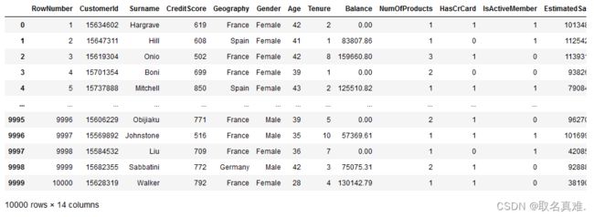
数据处理:
#Create dummy variables 机器不能识别字符,转为数字
geography=pd.get_dummies(X["Geography"],drop_first=True)
gender=pd.get_dummies(X['Gender'],drop_first=True)

## Concatenate the Data Frames

X=pd.concat([X,geography,gender],axis=1)

## Drop Unnecessary columns
X=X.drop(['Geography','Gender'],axis=1)
随机森林建模:
# Splitting the dataset into the Training set and Test set
from sklearn.model_selection import train_test_split
X_train, X_test, y_train, y_test = train_test_split(X, y, test_size = 0.3, random_state = 0)

from sklearn.ensemble import RandomForestClassifier
classifier=RandomForestClassifier()
classifier.fit(X_train,y_train)

y_pred=classifier.predict(X_test)
#Import scikit-learn metrics module for accuracy calculation
from sklearn import metrics

# Model Accuracy, how often is the classifier correct?
print("Accuracy:",metrics.accuracy_score(y_test, y_pred))
#结果:Accuracy: 0.8646666666666667
LIME
import pickle
pickle.dump(classifier, open("classifier.pkl", 'wb'))

classifier1=pd.read_pickle('classifier.pkl')

import lime
from lime import lime_tabular

interpretor = lime_tabular.LimeTabularExplainer(
    training_data=np.array(X_train),#用于训练解释模型的样本数据。
    feature_names=X_train.columns,#具有特征名称的特征的列表。
    mode='classification'#解释模型的模式,默认为 "classification",也可以设置为 "regression"。
)

# feature importance of the random forest model
feature_importance = pd.DataFrame()
feature_importance['variable'] = X_train.columns
feature_importance['importance'] = classifier1.feature_importances_

# feature_importance values in descending order
feature_importance.sort_values(by='importance', ascending=False).head(10)#该模型权重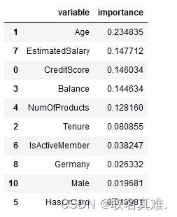
例一:
X_test.iloc[88]
'''结果:
CreditScore           756.00
Age                    39.00
Tenure                  3.00
Balance            100717.85
NumOfProducts           3.00
HasCrCard               1.00
IsActiveMember          1.00
EstimatedSalary     73406.04
Germany                 1.00
Spain                   0.00
Male                    0.00
Name: 1096, dtype: float64
'''

print('prediction: {}'.format(classifier1.predict(X_test.iloc[[88],:])))
#结果:prediction: [1]

exp = interpretor.explain_instance(
    data_row=X_test.iloc[88], ##new data要解释的实例数据
    predict_fn=classifier1.predict_proba#: 用于预测的函数。
)

exp.show_in_notebook(show_table=True)#该人可能属于流失或不流失的概率及各特征占比可能性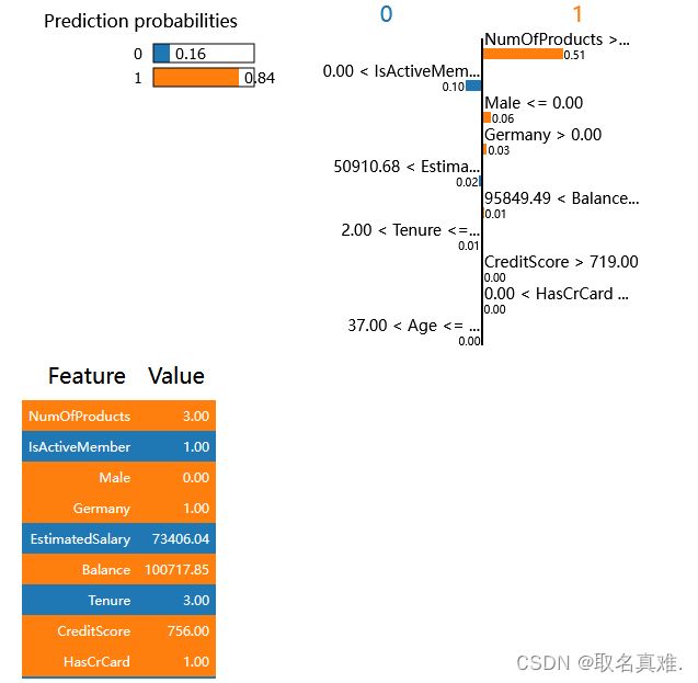
exp.as_pyplot_figure() 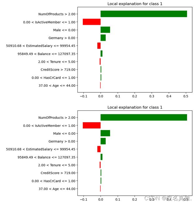
例二:
exp = interpretor.explain_instance(
    data_row=X_test.iloc[2], ##new data
    predict_fn=classifier1.predict_proba,
    num_features=10
)

X_test.iloc[2]
'''结果:
CreditScore          706.00
Age                   42.00
Tenure                 8.00
Balance            95386.82
NumOfProducts          1.00
HasCrCard              1.00
IsActiveMember         1.00
EstimatedSalary    75732.25
Germany                0.00
Spain                  1.00
Male                   0.00
Name: 2398, dtype: float64
'''

exp.show_in_notebook(show_table=True,show_all=False)
exp.as_pyplot_figure() 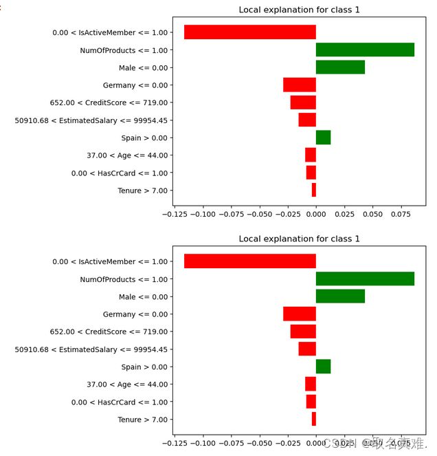
exp.as_list()
'''结果:
[('0.00 < IsActiveMember <= 1.00', -0.11661097094408614),
('NumOfProducts <= 1.00', 0.08686460877739129),
('Male <= 0.00', 0.043159886277428304),
('Germany <= 0.00', -0.029197882161009953),
('652.00 < CreditScore <= 719.00', -0.022598898299313823),
('50910.68 < EstimatedSalary <= 99954.45', -0.01532003910694092),
('Spain > 0.00', 0.013041709019348565),
('37.00 < Age <= 44.00', -0.009812578647407045),
('0.00 < HasCrCard <= 1.00', -0.008498455231089774),
('Tenure > 7.00', -0.0038766005937966638)]
'''