电子商务平台拍卖数据分析实战 scikit-learn 实现数据分析

内容简介

        风风火火的双十一过去了，今年的你又给某宝剁了多少手，拔了多少草呢。本节课程我们将介绍另外一个国际贸易门户 --ebay，一个致力于为中国商家开辟海外网络直销渠道的平台。我们可以在这个平台上充当买家或是卖家。与淘宝不同的是，这个平台不是一口价交易，而是设置一个开始竞投的价格后开始拍卖。
       我们就是要利用 ebay 上的历史拍卖数据，用机器学习的方法来训练一个模型，以预测一项拍卖是否会成功，和成功的交易最终的成交价格

知识点

1.  学习如何用 scikit-learn 的机器学习算法
2. scikit-learn 做数据分析
3. 数据分析结果可视化

在线拍卖数据初步分析

ebay在线拍卖数据

我们运用的 ebay 在线拍卖数 数据集为 Ebay Data Set，这个数据是由 Jay Grossman 提供的。这个数据集是由一个为运动爱好者提供资讯的平台 SportsCollector。

数据集 raw.tar.gz 数据中包括 TrainingSet.csv，TestSet.csv .TrainingSubset.csv和 TestSubset.csv下表中列出了这四个文件的内容简介:

数据名	数据描述	数据量
Training Set	2013 年 4 月的所有拍卖	25，8588
Test Set	2013 年5月第一个周的所有拍卖	3，7460
Training Subset	2013 年 4 月成功交易的所有拍卖	7,9732
Test Subset	2013 年5月第一周成功交易的所有拍卖	9392

表示数据的 特征向量 中的特征名及其对应性质:

数据准备及环境配置

首先，通过 wget命令获取本次数据分析的 ebay 拍卖数据 raw.tar.gz ，并解压数据。

!wget -nc http://labfile.oss.aliyuncs.com/courses/714/raw.tar.gz

!tar zxvf raw.tar.gz

数据可视化

接下来，导入相关的包：

import pandas as pd
from pandas import DataFrame
import numpy as np
%matplotlib inline
from matplotlib import pyplot as plt
import seaborn as sns

读入数据：

test_set = pd.read_csv('raw/TestSet.csv')
train_set = pd.read_csv('raw/TrainingSet.csv')
test_subset = pd.read_csv('raw/TestSubset.csv')
train_subset = pd.read_csv('raw/TrainingSubset.csv')

第一列属性 EbayID 为每条拍卖记录的 D 号，与预测拍卖是否成功没有联系，因此在模型训练时将该特征去除。ouantitysold 属性为 1 时代表拍卖成功，为 0 时代表拍卖失败，其中 sellerName 拍卖卖方的名字与预测拍卖是否成功时没有多大的关系，因此在训练时也将该特征去除。

train = train_set.drop(['EbayID','QuantitySold','SellerName'], axis=1)
train_target = train_set['QuantitySold']

# 获取总特征数
_, n_features = train.shape

可视化数据，取出一部分特征，两两组成对看数据在这个 2 维平面上的分布情况

# isSold： 拍卖成功为1， 拍卖失败为0

df = DataFrame(np.hstack((train,train_target[:, None])), columns=list(range(n_features)) + ["isSold"])
_ = sns.pairplot(df[:50], vars=[2,3,4,10,13], hue="isSold", size=1.5)

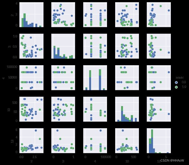
从第 3,9,12,16 维特征的散列图及柱状图可看出，这几个维度并不是有很好地区分度，横坐标的值分别代表不同维度之间的正负相关性，为了查看数据特征之间的相关性，及不同特征与类别 ssold 之间的关系，我们可以利用 seaborn 中的热度图来显示其两两组队之间的相关性

plt.figure(figsize=(10,10))

# 计算数据的相关性矩阵
corr = df.corr()

# 产生遮挡出热度图上三角部分的mask，因为这个热度图为对称矩阵，所以只输出下三角部分即可
mask = np.zeros_like(corr,dtype=np.bool)
mask[np.triu_indices_from(mask)] = True

# 产生热度图中对应的变化的颜色
cmap = sns.diverging_palette(220, 10, as_cmap=True)

# 调用seanborn中的heat创建热度图
sns.heatmap(corr, mask=mask, cmap=cmap, vmax = .3,
                square=True, xticklabels=5, yticklabels=2,
                linewidths=.5, cbar_kws={"shrink":.5})

# 将yticks旋转至水平方向，方便查看
plt.yticks(rotation=0)

plt.show()

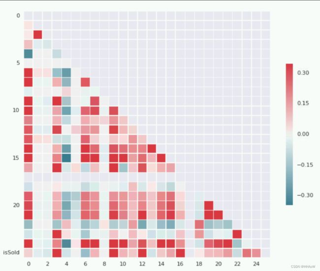
        上幅图中，颜色越偏向红色的相关性越大，越偏向蓝色的相关性越小且负相关，白色即两个特征之间没有多大的关联。
        通过最后一行可看出，不同维的属性与类别 issold 之间的关系
        其中第 3,9,12,16 维特征与拍卖是否会成功有很强的 正相关性，其中 3,9,12,16 分别对应属性 SellerClosePercent 、HitCount、SellerSaleAvgPriceRatio 和 Bestoffer ，表示当这些属性的值越大时越有可能使拍卖成功。
        其中第 6 维特征 startingBid 与成功拍卖 issold 之间的呈现较大的负相关性，可看出当拍卖投标的底线越高则这项拍卖的成功性就越低。
        通过这幅热度图的第一列我们还可以看出不同特征与价格 rice 之间的相关性。同样的我们可以根据这些相关性，选出比较有利于我实现第二个任务-拍卖价格预测的特征

利用数据预测拍卖是否会成功

        由于我们的数据量比较大，且特征维度也不是特别少，因此我们一开始做 baseline 时，就不利用 SVM 支持向量机 这些较简单的模型因为当数据量比较大，且维度较高时，有些简单的机器学习算法就并不是很高效，且可能训练到最后都不收敛并耗时。

根据 scikit-learn 提供的 机器学习算法使用图谱:

scikit-learn 官方介绍 —— 机器学习使用图谱

        我们根据图谱推荐先使用SGDClassifier，其全称为 stochastic Gradient Descent 随机梯度下降 ，通过 梯度下降法 在训练过程中优化目标函数使得预测值与真实值之间的误差loss 最小化。
        SGDclassifier 每次练过程没有用到所有的训练样本，而是随机的从训练样本中选取一部分进行训练。
        而且 SGD 对特征值的大小比较敏感，而通过上面的数据展示，可以知道在我们的数据集里有数值较大的数据，如: category 。
        因此我们可以先用 sklearn.preprocessing 中提供的 standardScaler 对数据进行预处理，使其每个属性的波动幅度不要太大，有助于训练时函数收敛
        以下就是我们使用 sklearn 中的 SGDcassifier 实现拍卖是否成功的模型训练代码:

from sklearn.linear_model import SGDClassifier
from sklearn.preprocessing import StandardScaler

# prepare data
test_set = pd.read_csv('raw/TestSet.csv')
train_set = pd.read_csv('raw/TrainingSet.csv')

train = train_set.drop(['EbayID','QuantitySold','SellerName'], axis=1)
train_target = train_set['QuantitySold']

n_trainSamples, n_features = train.shape

# 画出训练过程中SGDClassifier利用不同的mini_batch学习的效果
def plot_learning(clf,title):

    plt.figure()
    # 记录上一次训练结果在本次batch上的预测情况
    validationScore = []
    # 记录加上本次batch训练结果后的预测情况
    trainScore = []
    # 最小训练批数
    mini_batch = 1000

    for idx in range(int(np.ceil(n_trainSamples / mini_batch))):
        x_batch = train[idx * mini_batch: min((idx + 1) * mini_batch, n_trainSamples)]
        y_batch = train_target[idx * mini_batch: min((idx + 1) * mini_batch, n_trainSamples)]

        if idx > 0:
            validationScore.append(clf.score(x_batch, y_batch))
        clf.partial_fit(x_batch, y_batch, classes=range(5))
        if idx > 0:
            trainScore.append(clf.score(x_batch, y_batch))
    plt.plot(trainScore, label="train score")
    plt.plot(validationScore, label="validation socre")
    plt.xlabel("Mini_batch")
    plt.ylabel("Score")
    plt.legend(loc='best')
    plt.grid()
    plt.title(title)

# 对数据进行归一化
scaler = StandardScaler()
train = scaler.fit_transform(train)
# 创建SGDClassifier
clf = SGDClassifier(penalty='l2', alpha=0.001)
plot_learning(clf,"SGDClassifier")

plt.show()

训练结果如下图，由于 SGDclassifier 的训练集是在所有的训练样本中抽取一部分作为本次的训练集，因此在这里不适用交叉验证。

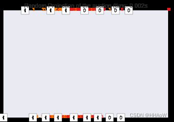
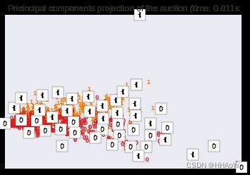
可看到 SGclassifier 的训练效果还不错，我们也可以通过 scikit-learn中封装的一些降维方法，将 数据可视化，这里我们使用的三种方法进行降维RandomProjection ，PCA 和 T-SNE embedding 。

from sklearn import (manifold, decomposition, random_projection)
from matplotlib import offsetbox
from time import time

# image[0]为数字0表示某条数据的isSold为0

images= []
images.append([[  0. ,   0. ,   5. ,  13. ,   9. ,   1. ,   0. ,   0. ],
 [  0. ,   0. ,  13. ,  15. ,  10. ,  15. ,   5. ,   0. ],
 [  0. ,   3. ,  15. ,   2. ,   0. ,  11. ,   8. ,   0. ],
 [  0. ,   4. ,  12. ,   0. ,   0. ,   8. ,   8. ,   0. ],
 [  0. ,   5. ,   8. ,   0. ,   0. ,   9. ,   8. ,   0. ],
 [  0. ,   4. ,  11. ,   0. ,   1. ,  12. ,   7. ,   0. ],
 [  0. ,   2. ,  14. ,   5. ,  10. ,  12. ,   0. ,   0. ],
 [  0. ,   0. ,   6. ,  13. ,  10. ,   0. ,   0. ,   0. ]])
 
# image[1]为数字1表示某条数据的isSold为1

images.append([[  0. ,   0. ,   0. ,  12. ,  13. ,   5. ,   0. ,   0. ],
 [  0. ,   0. ,   0. ,  11. ,  16. ,   9. ,   0. ,   0. ],
 [  0. ,   0. ,   3. ,  15. ,  16. ,   6. ,   0. ,   0. ],
 [  0. ,   7. ,  15. ,  16. ,  16. ,   2. ,   0. ,   0. ],
 [  0. ,   0. ,   1. ,  16. ,  16. ,   3. ,   0. ,   0. ],
 [  0. ,   0. ,   1. ,  16. ,  16. ,   6. ,   0. ,   0. ],
 [  0. ,   0. ,   1. ,  16. ,  16. ,   6. ,   0. ,   0. ],
 [  0. ,   0. ,   0. ,  11. ,  16. ,  10. ,   0. ,   0. ]])


# 这里只选取了1000条数据进行数据可视化展示

show_instancees = 1000

# define the drawing function

def plot_embedding(X, title=None):
    x_min, x_max = np.min(X, 0), np.max(X, 0)
    X = (X - x_min) / (x_max - x_min)

    plt.figure()
    ax = plt.subplot(111)
    for i in range(X.shape[0]):
        plt.text(X[i,0], X[i,1], str(train_target[i]),
                 color=plt.cm.Set1(train_target[i] / 2.),
                 fontdict={'weight':'bold','size':9})

    if hasattr(offsetbox, 'AnnotationBbox'):
        shown_images = np.array([[1., 1.]])  # just something big
    for i in range(show_instancees):
        dist = np.sum((X[i] - shown_images) ** 2, 1)
        if np.min(dist) < 4e-3:
            # don't show points that are too close
            continue
        shown_images = np.r_[shown_images, [X[i]]]
        auctionbox = offsetbox.AnnotationBbox(
            offsetbox.OffsetImage(images[train_target[i]], cmap=plt.cm.gray_r), X[i])
        ax.add_artist(auctionbox)
    plt.xticks([]), plt.yticks([])
    if title is not None:
        plt.title(title)

# 随机投影 Random Projection

start_time = time()
rp = random_projection.SparseRandomProjection(n_components=2, random_state=42)
rp.fit(train[:show_instancees])
train_projected = rp.transform(train[:show_instancees])
plot_embedding(train_projected, "Random Projection of the auction (time: %.3fs" % (time() - start_time))

# 主成分提取 PCA

start_time = time()
train_pca = decomposition.TruncatedSVD(n_components=2).fit_transform(train[:show_instancees])
plot_embedding(train_pca, "Pricincipal components projection of the auction (time: %.3fs" % (time() - start_time))

# t-sne 降维

start_time = time()
tsne = manifold.TSNE(n_components=2, init='pca', random_state=0)
train_tsne = tsne.fit_transform(train[:show_instancees])
plot_embedding(train_tsne, "T-SNE embedding of the auction (time: %.3fs" % (time() - start_time))

随机投影效果：

PCA降维效果：

t-sne降维效果：

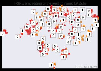
        从以上三幅图中，我们可以根据数字 0 和 1 的重叠情况，判读出我们的数据可区分度并不是特别大。

        因此我们的训练效果也没有达到特别好，从这方面也可以看出我们这里用来训练分类器的特征并不是利用得特别好。

        有兴趣的同学可以多了解下 特征工程，或者根据我们上面绘制的热度图挑选一些特征进行分类器训练，查看训练效果。

分类器训练结束后，可查看分类器在测试集上的测试效果：

# 导入相关包

from sklearn.metrics import (precision_score, recall_score, f1_score)

# 首先也是准备好测试数据，进行归一化处理

test = test_set.drop(['EbayID','QuantitySold','SellerName'],axis=1)
test_target = test_set['QuantitySold']
test = scaler.fit_transform(test)

# 利用训练好的分类器进行预测

test_pred = clf.predict(test) 

print("SGDClassifier training performance on testing dataset:" )
print("\tPrecision: %1.3f " % precision_score(test_target, test_pred))
print("\tRecall: %1.3f" % recall_score(test_target, test_pred))
print("\tF1: %1.3f \n" % f1_score(test_target, test_pred))

测试结果：

SGDClassifier training performance on testing dataset:
    Precision: 0.822 
    Recall: 0.736
    F1: 0.777 

预测拍卖最终成交价格

        由于在价格的分布是在一个连续的区间上，因此这与预测拍卖是否会成功是不同的，预测价格是一个 回归 预测，而判断拍卖是否会成功是一个 分类 任务
        同样根据 机器学习算法使用图谱，在这里我们采取 SGDRegressor其他使用情况与预测拍卖是否成功时差不多,代码如下:

from sklearn.linear_model import SGDRegressor
import random
from sklearn.preprocessing import MinMaxScaler

# prepare data
test_subset = pd.read_csv('raw/TestSubset.csv')
train_subset = pd.read_csv('raw/TrainingSubset.csv')

# 训练集
train = train_subset.drop(['EbayID','Price','SellerName'],axis=1)
train_target = train_subset['Price']

scaler = MinMaxScaler()
train = scaler.fit_transform(train)
n_trainSamples, n_features = train.shape

# ploting example from scikit-learn
def plot_learning(clf,title):

    plt.figure()
    validationScore = []
    trainScore = []
    mini_batch = 500
    # define the shuffle index
    ind = list(range(n_trainSamples))
    random.shuffle(ind)

    for idx in range(int(np.ceil(n_trainSamples / mini_batch))):
        x_batch = train[ind[idx * mini_batch: min((idx + 1) * mini_batch, n_trainSamples)]]
        y_batch = train_target[ind[idx * mini_batch: min((idx + 1) * mini_batch, n_trainSamples)]]

        if idx > 0:
            validationScore.append(clf.score(x_batch, y_batch))
        clf.partial_fit(x_batch, y_batch)
        if idx > 0:
            trainScore.append(clf.score(x_batch, y_batch))

    plt.plot(trainScore, label="train score")
    plt.plot(validationScore, label="validation socre")
    plt.xlabel("Mini_batch")
    plt.ylabel("Score")
    plt.legend(loc='best')
    plt.title(title)

sgd_regresor = SGDRegressor(penalty='l2',alpha=0.001)
plot_learning(sgd_regresor,"SGDRegressor")

# 准备测试集查看测试情况
test = test_subset.drop(['EbayID','Price','SellerName'],axis=1)
test = scaler.fit_transform(test)
test_target = test_subset['Price']

print("SGD regressor prediction result on testing data: %.3f" % sgd_regresor.score(test,test_target))

plt.show()

训练过程：

        在测试集上的测试结果:SGD regressor prediction result on testing data:0.93 由于 SGDRegressor 的回归效果还不错，因此我们没有在进一步的选择其他的模型进行尝试，有兴趣的同学可以在这方面在多改进参数，或者尝试其他的方法看预测效果如何。

总结

        我们学习了如何使用 sikit-learn 进行数据分析，其实在数据分析过程中，运用到 机器学习 的算法进行模型训练并不是最主要的，很多时候是如何在前期进行数据 预处理。
        这过程中包括数据的筛选，和 特征工程 等，在进行一项 数据挖掘 任务时，我们可能会花更多的时间在数据 预处理 和 特征工程 上，但是这些准备工作做好后，可使得我们之后的模型训练过程事半功倍
        在 scikit-learn 官方文档中也有许多数据库和算法实现例子，并且有很多 数据可视化 的例子，运用这些例子也能帮助我们快速入门 机器学习 这个领域