cs231n assignment1——SVM
整体思路
- 加载CIFAR-10数据集并展示部分数据
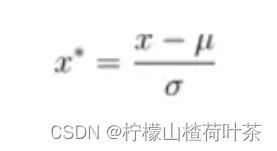
- 数据图像归一化,减去均值(也可以再除以方差)
- svm_loss_naive和svm_loss_vectorized计算hinge损失,用拉格朗日法列hinge损失函数
- 利用随机梯度下降法优化SVM
- 在训练集和验证集计算准确率,保存最好的模型在测试集进行预测计算准确率
加载展示划分数据集
加载CIFAR-10数据集
# Load the raw CIFAR-10 data.
#加载CIFAR-10数据集
cifar10_dir = 'cs231n/datasets/cifar-10-batches-py'

# Cleaning up variables to prevent loading data multiple times (which may cause memory issue)
#清理变量以防止多次加载数据
try:
   del X_train, y_train
   del X_test, y_test
   print('Clear previously loaded data.')
except:
   pass

X_train, y_train, X_test, y_test = load_CIFAR10(cifar10_dir)

# As a sanity check, we print out the size of the training and test data.
#打印出训练和测试数据的大小。
print('Training data shape: ', X_train.shape)
print('Training labels shape: ', y_train.shape)
print('Test data shape: ', X_test.shape)
print('Test labels shape: ', y_test.shape)
# Visualize some examples from the dataset.
#可视化部分数据
# We show a few examples of training images from each class.
#从每个类别中展示一些训练图片
classes = ['plane', 'car', 'bird', 'cat', 'deer', 'dog', 'frog', 'horse', 'ship', 'truck']
num_classes = len(classes)
samples_per_class = 7
for y, cls in enumerate(classes):
    idxs = np.flatnonzero(y_train == y)
    idxs = np.random.choice(idxs, samples_per_class, replace=False)
    for i, idx in enumerate(idxs):
        plt_idx = i * num_classes + y + 1
        plt.subplot(samples_per_class, num_classes, plt_idx)
        plt.imshow(X_train[idx].astype('uint8'))
        plt.axis('off')
        if i == 0:
            plt.title(cls)
plt.show()
划分数据集
# Split the data into train, val, and test sets. In addition we will
# create a small development set as a subset of the training data;
# we can use this for development so our code runs faster.
#将数据集划分为训练集49000张,测试集1000张和验证集1000张
#创建小样本数据加速训练
num_training = 49000
num_validation = 1000
num_test = 1000
num_dev = 500

# Our validation set will be num_validation points from the original
# training set.
#验证集取自原始训练集
mask = range(num_training, num_training + num_validation)
X_val = X_train[mask]
y_val = y_train[mask]

# Our training set will be the first num_train points from the original
# training set.
#训练集也取自原始训练集
mask = range(num_training)
X_train = X_train[mask]
y_train = y_train[mask]

# We will also make a development set, which is a small subset of
# the training set.
mask = np.random.choice(num_training, num_dev, replace=False)
X_dev = X_train[mask]
y_dev = y_train[mask]

# We use the first num_test points of the original test set as our
# test set.
mask = range(num_test)
X_test = X_test[mask]
y_test = y_test[mask]

print('Train data shape: ', X_train.shape)
print('Train labels shape: ', y_train.shape)
print('Validation data shape: ', X_val.shape)
print('Validation labels shape: ', y_val.shape)
print('Test data shape: ', X_test.shape)
print('Test labels shape: ', y_test.shape)
数据集格式转换
# Preprocessing: reshape the image data into rows
#将图像数据转化为行
X_train = np.reshape(X_train, (X_train.shape[0], -1))
X_val = np.reshape(X_val, (X_val.shape[0], -1))
X_test = np.reshape(X_test, (X_test.shape[0], -1))
X_dev = np.reshape(X_dev, (X_dev.shape[0], -1))

# As a sanity check, print out the shapes of the data
#输出数据集形状
print('Training data shape: ', X_train.shape)
print('Validation data shape: ', X_val.shape)
print('Test data shape: ', X_test.shape)
print('dev data shape: ', X_dev.shape)
图像数据归一化
# Preprocessing: subtract the mean image
#减去均值
# first: compute the image mean based on the training data
#计算训练数据的均值
mean_image = np.mean(X_train, axis=0)
print(mean_image[:10]) # 输出部分元素
plt.figure(figsize=(4,4))
plt.imshow(mean_image.reshape((32,32,3)).astype('uint8')) # visualize the mean image
plt.show()

# second: subtract the mean image from train and test data
#减去均值(更严谨的话可以继续除以方差)
X_train -= mean_image
X_val -= mean_image
X_test -= mean_image
X_dev -= mean_image

# third: append the bias dimension of ones (i.e. bias trick) so that our SVM
# only has to worry about optimizing a single weight matrix W.
#数据维度转变简便计算优化权重矩阵W
X_train = np.hstack([X_train, np.ones((X_train.shape[0], 1))])
X_val = np.hstack([X_val, np.ones((X_val.shape[0], 1))])
X_test = np.hstack([X_test, np.ones((X_test.shape[0], 1))])
X_dev = np.hstack([X_dev, np.ones((X_dev.shape[0], 1))])

print(X_train.shape, X_val.shape, X_test.shape, X_dev.shape)
评估多类 SVM 损失函数的函数

(图来自《从零开始:机器学习的数学原理和算法实践》)

所以我们在linear_svm.py中完善svm_loss_naive
def svm_loss_naive(W, X, y, reg):
    """
    Structured SVM loss function, naive implementation (with loops).

    Inputs have dimension D, there are C classes, and we operate on minibatches
    of N examples.

    Inputs:
    - W: A numpy array of shape (D, C) containing weights.
    - X: A numpy array of shape (N, D) containing a minibatch of data.
    - y: A numpy array of shape (N,) containing training labels; y[i] = c means
      that X[i] has label c, where 0 <= c < C.
    - reg: (float) regularization strength

    Returns a tuple of:
    - loss as single float
    - gradient with respect to weights W; an array of same shape as W
    """
    #梯度矩阵初始化
    dW = np.zeros(W.shape)  # initialize the gradient as zero

    # compute the loss and the gradient
    #计算损失和梯度
    num_classes = W.shape[1]
    num_train = X.shape[0]
    loss = 0.0
    for i in range(num_train):
        #W*Xi
        score = X[i].dot(W)
        correct_score = score[y[i]]
        for j in range(num_classes):
            #预测正确
            if j == y[i]:
                continue
            #W*Xi-Wyi*Xi+1
            margin = score[j] - correct_score + 1  # 拉格朗日
            if margin > 0:
                loss += margin

    # Right now the loss is a sum over all training examples, but we want it
    # to be an average instead so we divide by num_train.
    #平均损失
    loss /= num_train
	#加上正则化λ||W||²
    # Add regularization to the loss.
    loss += reg * np.sum(W * W)

    #############################################################################
    # TODO:                                                                     #
    # Compute the gradient of the loss function and store it dW.                #
    # Rather that first computing the loss and then computing the derivative,   #
    # it may be simpler to compute the derivative at the same time that the     #
    # loss is being computed. As a result you may need to modify some of the    #
    # code above to compute the gradient.                                       #
    #############################################################################
    # *****START OF YOUR CODE (DO NOT DELETE/MODIFY THIS LINE)*****

    dW /= num_train

    dW += reg * W

    # *****END OF YOUR CODE (DO NOT DELETE/MODIFY THIS LINE)*****

    return loss, dW
评估svm_loss_naive函数
# Evaluate the naive implementation of the loss we provided for you:
from cs231n.classifiers.linear_svm import svm_loss_naive
import time

# generate a random SVM weight matrix of small numbers
# 随机初始化权重矩阵
W = np.random.randn(3073, 10) * 0.0001
#计算梯度和损失
loss, grad = svm_loss_naive(W, X_dev, y_dev, 0.000005)
print('loss: %f' % (loss, ))
在验证集计算梯度损失
数值估计损失函数的梯度,并将数值估计值与计算的梯度进行比较
# Once you've implemented the gradient, recompute it with the code below
# and gradient check it with the function we provided for you

# Compute the loss and its gradient at W.
#计算损失和梯度
loss, grad = svm_loss_naive(W, X_dev, y_dev, 0.0)

# Numerically compute the gradient along several randomly chosen dimensions, and
# compare them with your analytically computed gradient. The numbers should match
# almost exactly along all dimensions.
from cs231n.gradient_check import grad_check_sparse
f = lambda w: svm_loss_naive(w, X_dev, y_dev, 0.0)[0]
grad_numerical = grad_check_sparse(f, W, grad)

# do the gradient check once again with regularization turned on
# you didn't forget the regularization gradient did you?
loss, grad = svm_loss_naive(W, X_dev, y_dev, 5e1)
f = lambda w: svm_loss_naive(w, X_dev, y_dev, 5e1)[0]
grad_numerical = grad_check_sparse(f, W, grad)
用向量形式计算损失函数

所以我们在linear_svm.py中完善svm_loss_vectorized
def svm_loss_vectorized(W, X, y, reg):
    """
    Structured SVM loss function, vectorized implementation.

    Inputs and outputs are the same as svm_loss_naive.
    """
    loss = 0.0
    dW = np.zeros(W.shape)  # initialize the gradient as zero

    #############################################################################
    # TODO:                                                                     #
    # Implement a vectorized version of the structured SVM loss, storing the    #
    # result in loss.                                                           #
    #############################################################################
    # *****START OF YOUR CODE (DO NOT DELETE/MODIFY THIS LINE)*****

    num_train=X.shape[0]
    classes_num=X.shape[1]

    score = X.dot(W)
    #矩阵大小变化,大小不同的矩阵不可以加减
    correct_scores = score[range(num_train), list(y)].reshape(-1, 1) #[N, 1]
    margin = np.maximum(0, score - correct_scores + 1)
    margin[range(num_train), list(y)] = 0
    #正则化
    loss = np.sum(margin) / num_train
    loss += 0.5 * reg * np.sum(W * W)

    # *****END OF YOUR CODE (DO NOT DELETE/MODIFY THIS LINE)*****

    #############################################################################
    # TODO:                                                                     #
    # Implement a vectorized version of the gradient for the structured SVM     #
    # loss, storing the result in dW.                                           #
    #                                                                           #
    # Hint: Instead of computing the gradient from scratch, it may be easier    #
    # to reuse some of the intermediate values that you used to compute the     #
    # loss.                                                                     #
    #############################################################################
    # *****START OF YOUR CODE (DO NOT DELETE/MODIFY THIS LINE)*****
    #大于0的置1,其余为0
    margin[margin>0] = 1
    margin[range(num_train),list(y)] = 0

    margin[range(num_train),y] -= np.sum(margin,1)

    dW=X.T.dot(margin)

    dW=dW/num_train
    dW=dW+reg*W


    # *****END OF YOUR CODE (DO NOT DELETE/MODIFY THIS LINE)*****

    return loss, dW
然后我们对比两种损失函数计算的时间差异
# Complete the implementation of svm_loss_vectorized, and compute the gradient
# of the loss function in a vectorized way.

# The naive implementation and the vectorized implementation should match, but
# the vectorized version should still be much faster.
tic = time.time()
_, grad_naive = svm_loss_naive(W, X_dev, y_dev, 0.000005)
toc = time.time()
print('Naive loss and gradient: computed in %fs' % (toc - tic))

tic = time.time()
_, grad_vectorized = svm_loss_vectorized(W, X_dev, y_dev, 0.000005)
toc = time.time()
print('Vectorized loss and gradient: computed in %fs' % (toc - tic))

# The loss is a single number, so it is easy to compare the values computed
# by the two implementations. The gradient on the other hand is a matrix, so
# we use the Frobenius norm to compare them.
difference = np.linalg.norm(grad_naive - grad_vectorized, ord='fro')
print('difference: %f' % difference)
使用SGD优化

from __future__ import print_function

from builtins import range
from builtins import object
import numpy as np
from ..classifiers.linear_svm import *
from ..classifiers.softmax import *
from past.builtins import xrange


class LinearClassifier(object):
    def __init__(self):
        self.W = None

    def train(
        self,
        X,
        y,
        learning_rate=1e-3,
        reg=1e-5,
        num_iters=100,
        batch_size=200,
        verbose=False,
    ):
        """
        Train this linear classifier using stochastic gradient descent.

        Inputs:
        - X: A numpy array of shape (N, D) containing training data; there are N
          training samples each of dimension D.
        - y: A numpy array of shape (N,) containing training labels; y[i] = c
          means that X[i] has label 0 <= c < C for C classes.
        - learning_rate: (float) learning rate for optimization.
        - reg: (float) regularization strength.
        - num_iters: (integer) number of steps to take when optimizing
        - batch_size: (integer) number of training examples to use at each step.
        - verbose: (boolean) If true, print progress during optimization.

        Outputs:
        A list containing the value of the loss function at each training iteration.
        """
        num_train, dim = X.shape
        num_classes = (
            np.max(y) + 1
        )  # assume y takes values 0...K-1 where K is number of classes
        if self.W is None:
            # lazily initialize W
            self.W = 0.001 * np.random.randn(dim, num_classes)

        # Run stochastic gradient descent to optimize W
        loss_history = []
        for it in range(num_iters):
            X_batch = None
            y_batch = None

            #########################################################################
            # TODO:                                                                 #
            # Sample batch_size elements from the training data and their           #
            # corresponding labels to use in this round of gradient descent.        #
            # Store the data in X_batch and their corresponding labels in           #
            # y_batch; after sampling X_batch should have shape (batch_size, dim)   #
            # and y_batch should have shape (batch_size,)                           #
            #                                                                       #
            # Hint: Use np.random.choice to generate indices. Sampling with         #
            # replacement is faster than sampling without replacement.              #
            #########################################################################
            # *****START OF YOUR CODE (DO NOT DELETE/MODIFY THIS LINE)*****
            hint=np.random.choice(num_train,batch_size,replace=True)
            X_batch = X[hint]
            y_batch = y[hint]


            # *****END OF YOUR CODE (DO NOT DELETE/MODIFY THIS LINE)*****

            # evaluate loss and gradient
            loss, grad = self.loss(X_batch, y_batch, reg)
            loss_history.append(loss)

            # perform parameter update
            #########################################################################
            # TODO:                                                                 #
            # Update the weights using the gradient and the learning rate.          #
            #########################################################################
            # *****START OF YOUR CODE (DO NOT DELETE/MODIFY THIS LINE)*****

            self.W = self.W - learning_rate * grad

            # *****END OF YOUR CODE (DO NOT DELETE/MODIFY THIS LINE)*****

            if verbose and it % 100 == 0:
                print("iteration %d / %d: loss %f" % (it, num_iters, loss))

        return loss_history

    def predict(self, X):
        """
        Use the trained weights of this linear classifier to predict labels for
        data points.

        Inputs:
        - X: A numpy array of shape (N, D) containing training data; there are N
          training samples each of dimension D.

        Returns:
        - y_pred: Predicted labels for the data in X. y_pred is a 1-dimensional
          array of length N, and each element is an integer giving the predicted
          class.
        """
        y_pred = np.zeros(X.shape[0])
        ###########################################################################
        # TODO:                                                                   #
        # Implement this method. Store the predicted labels in y_pred.            #
        ###########################################################################
        # *****START OF YOUR CODE (DO NOT DELETE/MODIFY THIS LINE)*****

        scores = X.dot(self.W)
        y_pred = y_pred+np.argmax(scores,1)

        # *****END OF YOUR CODE (DO NOT DELETE/MODIFY THIS LINE)*****
        return y_pred

    def loss(self, X_batch, y_batch, reg):
        """
        Compute the loss function and its derivative.
        Subclasses will override this.

        Inputs:
        - X_batch: A numpy array of shape (N, D) containing a minibatch of N
          data points; each point has dimension D.
        - y_batch: A numpy array of shape (N,) containing labels for the minibatch.
        - reg: (float) regularization strength.

        Returns: A tuple containing:
        - loss as a single float
        - gradient with respect to self.W; an array of the same shape as W
        """
        pass


class LinearSVM(LinearClassifier):
    """ A subclass that uses the Multiclass SVM loss function """

    def loss(self, X_batch, y_batch, reg):
        return svm_loss_vectorized(self.W, X_batch, y_batch, reg)


class Softmax(LinearClassifier):
    """ A subclass that uses the Softmax + Cross-entropy loss function """

    def loss(self, X_batch, y_batch, reg):
        return softmax_loss_vectorized(self.W, X_batch, y_batch, reg)
利用SGD迭代减少损失
from cs231n.classifiers import LinearSVM
#加载SVM
svm = LinearSVM()
tic = time.time()
loss_hist = svm.train(X_train, y_train, learning_rate=1e-7, reg=2.5e4,
                      num_iters=1500, verbose=True)
toc = time.time()
print('That took %fs' % (toc - tic))
在训练集和验证集计算准确率
#在训练集和验证集进行预测结果,计算准确率
y_train_pred = svm.predict(X_train)
print('training accuracy: %f' % (np.mean(y_train == y_train_pred), ))
y_val_pred = svm.predict(X_val)
print('validation accuracy: %f' % (np.mean(y_val == y_val_pred), ))
计算预测数据准确率
# Use the validation set to tune hyperparameters (regularization strength and
# learning rate). You should experiment with different ranges for the learning
# rates and regularization strengths; if you are careful you should be able to
# get a classification accuracy of about 0.39 (> 0.385) on the validation set.

# Note: you may see runtime/overflow warnings during hyper-parameter search.
# This may be caused by extreme values, and is not a bug.

# results is dictionary mapping tuples of the form
# (learning_rate, regularization_strength) to tuples of the form
# (training_accuracy, validation_accuracy). The accuracy is simply the fraction
# of data points that are correctly classified.
results = {}
best_val = -1   # The highest validation accuracy that we have seen so far.
best_svm = None # The LinearSVM object that achieved the highest validation rate.

################################################################################
# TODO:                                                                        #
# Write code that chooses the best hyperparameters by tuning on the validation #
# set. For each combination of hyperparameters, train a linear SVM on the      #
# training set, compute its accuracy on the training and validation sets, and  #
# store these numbers in the results dictionary. In addition, store the best   #
# validation accuracy in best_val and the LinearSVM object that achieves this  #
# accuracy in best_svm.                                                        #
#                                                                              #
# Hint: You should use a small value for num_iters as you develop your         #
# validation code so that the SVMs don't take much time to train; once you are #
# confident that your validation code works, you should rerun the validation   #
# code with a larger value for num_iters.                                      #
################################################################################

# Provided as a reference. You may or may not want to change these hyperparameters
#学习率
learning_rates = [1e-7, 5e-5]
#reg
regularization_strengths = [2.5e4, 5e4]

# *****START OF YOUR CODE (DO NOT DELETE/MODIFY THIS LINE)*****

for learning_rate in learning_rates:
  for regularization_strength in regularization_strengths:
    svm = LinearSVM()
    #svm训练
    loss_hist = svm.train(X_train, y_train, learning_rate=learning_rate, reg=regularization_strength, num_iters=1500, verbose=True)
    #在训练集预测,计算平均准确率
    y_train_pred2 = svm.predict(X_train)
    training_accuracy = np.mean(y_train == svm.predict(X_train))
    print('training accuracy: %f' % (np.mean(y_train == y_train_pred2)))
    #在验证集预测,计算平均准确率
    y_val_pred2 = svm.predict(X_val)
    val_accuracy = np.mean(y_val== svm.predict(X_val))
    print('validation accuracy: %f' % (np.mean(y_val == y_val_pred2)))
    #在训练集和验证集计算的准确率保存在results
    results[(learning_rate,regularization_strength)] = (training_accuracy,val_accuracy)
    print(results)
    #取最大的准确率保存在best_val
    if best_val < val_accuracy:
      best_val = val_accuracy
      best_svm = svm

# *****END OF YOUR CODE (DO NOT DELETE/MODIFY THIS LINE)*****

# Print out results.
for lr, reg in sorted(results):
    train_accuracy, val_accuracy = results[(lr, reg)]
    print('lr %e reg %e train accuracy: %f val accuracy: %f' % (
                lr, reg, train_accuracy, val_accuracy))

print('best validation accuracy achieved during cross-validation: %f' % best_val)
将最好的模型保存在best_svm中,在测试集计算准确率
# Evaluate the best svm on test set
y_test_pred = best_svm.predict(X_test)
test_accuracy = np.mean(y_test == y_test_pred)
print('linear SVM on raw pixels final test set accuracy: %f' % test_accuracy)
主要解决问题:
-
损失函数和梯度的推导
-
为什么SGD越迭代可能产生loss变大的情况:
因为SGD在每一步放弃了对梯度准确性的追求,每步仅仅随机采样少量样本来计算梯度,计算速度快,内存开销小,但是由于每步接受的信息量有限,对梯度的估计出现偏差也在所难免,造成目标函数曲线收敛轨迹显得很不稳定,伴有剧烈波动,甚至有时出现不收敛的情况。(这很正常!)
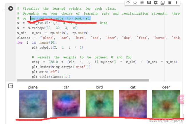
一个冷笑话(这能看出来是啥就有鬼了,果然用词很严谨
%f’ % (
lr, reg, train_accuracy, val_accuracy))
print(‘best validation accuracy achieved during cross-validation: %f’ % best_val)
将最好的模型保存在best_svm中,在测试集计算准确率

```python
# Evaluate the best svm on test set
y_test_pred = best_svm.predict(X_test)
test_accuracy = np.mean(y_test == y_test_pred)
print('linear SVM on raw pixels final test set accuracy: %f' % test_accuracy)
主要解决问题:
-
损失函数和梯度的推导
-
为什么SGD越迭代可能产生loss变大的情况:
因为SGD在每一步放弃了对梯度准确性的追求,每步仅仅随机采样少量样本来计算梯度,计算速度快,内存开销小,但是由于每步接受的信息量有限,对梯度的估计出现偏差也在所难免,造成目标函数曲线收敛轨迹显得很不稳定,伴有剧烈波动,甚至有时出现不收敛的情况。(这很正常!)
一个冷笑话(这能看出来是啥就有鬼了,果然用词很严谨