yolov5模型Detection输出内容与源码详细解读

---

前言

最近，需要修改yolov5推理结果，通过推理特征添加一些其它操作(如蒸馏)。显然，你需要对yolov5推理输出内容有详细了解，方可被你使用。为此，本文将记录个人对yolov5输出内容源码解读，这样对于你修改源码或蒸馏操作可提供理论参考。

---

一、Detiction类源码说明

yolov5的detection类输出包含2个部分，一个是训练的输出，一个是预测的输出。而我将在这里解释类参数与训练、预测输出内容。为什么我使用一篇文章来说明？显然是训练与预测输出内容与原始图像尺寸、模型尺寸、特征尺寸以及回归box含义与使用细节。

整体源码如下：

class Detect(nn.Module):
    stride = None  # strides computed during build
    onnx_dynamic = False  # ONNX export parameter

    def __init__(self, nc=80, anchors=(), ch=(), inplace=True):  # detection layer
        super().__init__()
        self.nc = nc  # number of classes
        self.no = nc + 5  # number of outputs per anchor
        self.nl = len(anchors)  # number of detection layers
        self.na = len(anchors[0]) // 2  # number of anchors
        self.grid = [torch.zeros(1)] * self.nl  # init grid
        self.anchor_grid = [torch.zeros(1)] * self.nl  # init anchor grid
        self.register_buffer('anchors', torch.tensor(anchors).float().view(self.nl, -1, 2))  # shape(nl,na,2)
        self.m = nn.ModuleList(nn.Conv2d(x, self.no * self.na, 1) for x in ch)  # output conv
        self.inplace = inplace  # use in-place ops (e.g. slice assignment)

    def forward(self, x):
        z = []  # inference output
        for i in range(self.nl):
            x[i] = self.m[i](x[i])  # conv
            bs, _, ny, nx = x[i].shape  # x(bs,255,20,20) to x(bs,3,20,20,85)
            x[i] = x[i].view(bs, self.na, self.no, ny, nx).permute(0, 1, 3, 4, 2).contiguous()

            if not self.training:  # inference
                if self.onnx_dynamic or self.grid[i].shape[2:4] != x[i].shape[2:4]:
                    self.grid[i], self.anchor_grid[i] = self._make_grid(nx, ny, i)

                y = x[i].sigmoid()
                if self.inplace:
                    y[..., 0:2] = (y[..., 0:2] * 2 - 0.5 + self.grid[i]) * self.stride[i]  # xy
                    y[..., 2:4] = (y[..., 2:4] * 2) ** 2 * self.anchor_grid[i]  # wh
                else:  # for YOLOv5 on AWS Inferentia https://github.com/ultralytics/yolov5/pull/2953
                    xy = (y[..., 0:2] * 2 - 0.5 + self.grid[i]) * self.stride[i]  # xy
                    wh = (y[..., 2:4] * 2) ** 2 * self.anchor_grid[i]  # wh
                    y = torch.cat((xy, wh, y[..., 4:]), -1)
                z.append(y.view(bs, -1, self.no))

        return x if self.training else (torch.cat(z, 1), x)

二、Detection类初始化参数解读

我已voc数据为例说明，voc数据类别为20。我将其具体解释注释其代码中，如下：

def __init__(self, nc=20, anchors=(), ch=(), inplace=True):  # detection layer
        super().__init__()
	 self.nc = nc  #   =20 类别数量
	 self.no = nc + 5  # =25 每个类别需添加位置与置信度
	 self.nl = len(anchors)  # =3 yolov5检测层为3，每层特征有一个anchor，可使用anchors替代 
	 self.na = len(anchors[0]) // 2  # =3 获得每个grid的anchor数量
	 self.grid = [torch.zeros(1)] * self.nl  # =[tensor([0.]), tensor([0.]), tensor([0.])]，初始化grid，后期会每个特征变成[1,3,feature_w,feature_h,2],共三个
	 self.anchor_grid = [torch.zeros(1)] * self.nl  # 初始化anchor grid，与上面self.grid类似，直白说就是占位初始化
	 self.register_buffer('anchors', torch.tensor(anchors).float().view(self.nl, -1, 2))  # 将anchors值变成shape(3,3,2)与对应格式
	 self.m = nn.ModuleList(nn.Conv2d(x, self.no * self.na, 1) for x in ch)  # 3个模型数据输出转换，每个特征图输出转换，
	 self.inplace = inplace  # use in-place ops (e.g. slice assignment)

anchors值如下:

  - [10,13, 16,30, 33,23]  # P3/8
  - [30,61, 62,45, 59,119]  # P4/16
  - [116,90, 156,198, 373,326]  # P5/32

self.m模块：

ModuleList(
  (0): Conv2d(320, 75, kernel_size=(1, 1), stride=(1, 1))
  (1): Conv2d(640, 75, kernel_size=(1, 1), stride=(1, 1))
  (2): Conv2d(1280, 75, kernel_size=(1, 1), stride=(1, 1))
)

其中ch是输入，与模型图像大小关联。

三、Detection的训练输出源码解读

为便于快速理解模型训练输出内容，我直接去掉推理输出代码，这样一目了然知道模型输出内容。

    def forward(self, x):
        z = []  # inference output
        for i in range(self.nl):
            x[i] = self.m[i](x[i])  # 预测输出
            bs, _, ny, nx = x[i].shape  # x(bs,255,20,20) to x(bs,3,20,20,85)
            x[i] = x[i].view(bs, self.na, self.no, ny, nx).permute(0, 1, 3, 4, 2).contiguous()    

        return x 

输出x值为三个特征层的值输出，都表示[batch,3,h,w,cls+5]，含义为batch size图像的h*w个像素有3个预测，每个预测都是类别概率、置信度与box位置。其输出如下：

注：特别说明，x输出都没有经过sigmoid函数。

四、Detection的预测输出源码解读

为便于快速理解模型推理输出内容，我直去掉不必要判断，给出推理输出代码，这样一目了然知道模型输出内容。

    def forward(self, x):
        z = []  # inference output
        for i in range(self.nl):
            x[i] = self.m[i](x[i])  # conv
            bs, _, ny, nx = x[i].shape  # x(bs,255,20,20) to x(bs,3,20,20,85)
            x[i] = x[i].view(bs, self.na, self.no, ny, nx).permute(0, 1, 3, 4, 2).contiguous()

          	 # inference
             if self.onnx_dynamic or self.grid[i].shape[2:4] != x[i].shape[2:4]:
                 self.grid[i], self.anchor_grid[i] = self._make_grid(nx, ny, i)

             y = x[i].sigmoid()
             if self.inplace:
                 y[..., 0:2] = (y[..., 0:2] * 2 - 0.5 + self.grid[i]) * self.stride[i]  # xy
                 y[..., 2:4] = (y[..., 2:4] * 2) ** 2 * self.anchor_grid[i]  # wh
             else:  # for YOLOv5 on AWS Inferentia https://github.com/ultralytics/yolov5/pull/2953
                 xy = (y[..., 0:2] * 2 - 0.5 + self.grid[i]) * self.stride[i]  # xy
                 wh = (y[..., 2:4] * 2) ** 2 * self.anchor_grid[i]  # wh
                 y = torch.cat((xy, wh, y[..., 4:]), -1)
             z.append(y.view(bs, -1, self.no))

        return   (torch.cat(z, 1), x)

1、self.grid内容解读

grid为网格，可以理解是对应特征图的网格，以第一个特征宽高为80说明，grid[0]存的是像素位置坐标如下tensort示意。相当于，每个batch的高宽对应像素重复3次分别从0到79的x坐标和y坐标得到grid。而grid有三个特征，其它二个特征图也是同样原理，如下图。

tensor([[[[[ 0.,  0.],
           [ 1.,  0.],
           [ 2.,  0.],
           ...,
           [77.,  0.],
           [78.,  0.],
           [79.,  0.]],

          [[ 0.,  1.],
           [ 1.,  1.],
           [ 2.,  1.],
           ...,
           [77.,  1.],
           [78.,  1.],
           [79.,  1.]],

          [[ 0.,  2.],
           [ 1.,  2.],
           [ 2.,  2.],
           ...,
           [77.,  2.],
           [78.,  2.],
           [79.,  2.]],

          ...,

2、xy/wh内容解读

yolov5在经历一次sigmoid为y = x[i].sigmoid()，获得dx、dy、dw、dh值(我暂时这么理解)，在使用以下代码实现在该特征图对应xy值与wh值。特别注意，假设该特征图是8080尺寸，仅是获得在该特征8080层恢复到模型输入特征图像尺寸，还未到原始图像输入尺寸。源码如下：

y[..., 0:2] = (y[..., 0:2] * 2 - 0.5 + self.grid[i]) * self.stride[i]  # xy
y[..., 2:4] = (y[..., 2:4] * 2) ** 2 * self.anchor_grid[i]  # wh

这里也说明一下，dw/dh转到对应尺寸是直接乘以self.anchor_grid，而self.anchor_grid保留是anchors值如下:

  - [10,13, 16,30, 33,23]  # P3/8
  - [30,61, 62,45, 59,119]  # P4/16
  - [116,90, 156,198, 373,326]  # P5/32

最终扩展到对应特征图维度，如下显示：

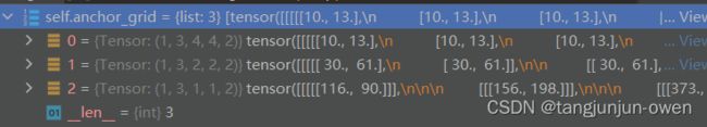
注：这里知道dx/dy/dw/dh恢复到模型输入尺寸(如640)即可。dw/dh并没有*strid，而是直接*anchors值。

3、推理输出解读

最后将输出内容通过view转换为[batch,-1,25]形式。

z.append(y.view(bs, -1, self.no))

即可获得(torch.cat(z, 1), x)这样的推理输出。我想说x实际还是训练输出内容，没有变化。

推理输出为2个列表，第一个列表就是上面说到的z值，其经历了sigmoid，包含类、置信度、box都使用了sigmoid，且box转为了模型输出对应尺寸位置。第二个列表为三个特征层的值输出，都表示[batch,3,h,w,cls+5]，含义为batch size图像的h*w个像素有3个预测，每个预测都是类别概率、置信度与box位置，是没有经历过sigmoid，实际就是训练输出内容。其结果示意如下：

注：x没有经过sigmoid，而z经过sigmoid后转成模型输出尺寸box。

---

总结

掌握yolov5的Detection类训练与预测输出内容，有利于对源码更改提供理论依据。