NLP学习笔记(为了完成基于知识图谱的问答系统进行的基础学习)
目录
- 前言
- 0.需要使用的模型的学习(更新中)
-
- Bi-LSTM
-
- 什么是LSTM与Bi-LSTM
- 为什么使用LSTM与Bi-LSTM
- LSTM
- 1. 一切的基础——词袋模型与句子相似度
-
- 词袋模型
- 句子相似度
- 简化:利用gensim
-
- 遇到的问题
- 2. TF-IDF——一个比较重要的原理
-
- 什么是TF-IDF
- 文本与预处理
- Gensim中的TF-IDF
- 实践计算TF-IDF值
- 第二部分的完整代码
- 3. 词形还原(Lemmatization)
-
- 什么是词形还原
- 指定单词词性
- 示例的Python代码
- 4. 命名实体识别(NER)
-
- 什么是NER
- 分类细节与工具
- 使用nltk实现NER
- 实现Stanford NER
前言
注意!这篇文章已经停止更新。
之后如果还有学习与分享需要,我会在新的文章里再写。
(毕竟这篇已经太长了)
这是笔者作为初学者在学习nlp时做的一些记录。部分图片、资料来自网络资源,如有不妥请评论区联系我修改或删除
0.需要使用的模型的学习(更新中)
Bi-LSTM
什么是LSTM与Bi-LSTM
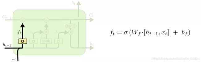
LSTM的全称是Long Short-Term Memory,它是RNN(Recurrent Neural Network)的一种。LSTM由于其设计的特点,非常适合用于对时序数据的建模,如文本数据。BiLSTM是Bi-directional Long Short-Term Memory的缩写,是由前向LSTM与后向LSTM组合而成。两者在自然语言处理任务中都常被用来建模上下文信息。
为什么使用LSTM与Bi-LSTM
将词的表示组合成句子的表示,可以采用相加的方法,即将所有词的表示进行加和,或者取平均等方法,但是这些方法没有考虑到词语在句子中前后顺序。如句子“我不觉得他好”。“不”字是对后面“好”的否定,即该句子的情感极性是贬义。使用LSTM模型可以更好的捕捉到较长距离的依赖关系。因为LSTM通过训练过程可以学到记忆哪些信息和遗忘哪些信息。
但是利用LSTM对句子进行建模还存在一个问题:无法编码从后到前的信息。在更细粒度的分类时,如对于强程度的褒义、弱程度的褒义、中性、弱程度的贬义、强程度的贬义的五分类任务需要注意情感词、程度词、否定词之间的交互。举一个例子,“这个餐厅脏得不行,没有隔壁好”,这里的“不行”是对“脏”的程度的一种修饰,通过BiLSTM可以更好的捕捉双向的语义依赖。
LSTM
-
总体

-
计算遗忘门
-
计算记忆门

-
计算当前时刻细胞状态

-
计算输出门和当前时刻隐层状态


1. 一切的基础——词袋模型与句子相似度
这一部分介绍NLP中常见的词袋模型(Bag of Words)以及如何利用词袋模型来计算句子间的相似度(余弦相似度,cosine similarity)
词袋模型
我们以下面两个简单句子为例:
sent1 = "I love sky, I love sea."
sent2 = "I like running, I love reading."
通常,NLP无法一下子处理完整的段落或句子,因此,第一步往往是分句和分词。这里只有句子,因此我们只需要分词即可。对于英语句子,可以使用NLTK中的word_tokenize函数,对于中文句子,则可使用jieba模块。故第一步为分词,代码如下:
from nltk import word_tokenize
sents = [sent1, sent2]
texts = [[word for word in word_tokenize(sent)] for sent in sents]
结果:
[['I', 'love', 'sky', ',', 'I', 'love', 'sea', '.'], ['I', 'like', 'running', ',', 'I', 'love', 'reading', '.']]
分词完毕。下一步是构建语料库,即所有句子中出现的单词及标点。代码如下:
all_list = []
for text in texts:
    all_list += text
corpus = set(all_list)
print(corpus)
结果:
{'love', 'running', 'reading', 'sky', '.', 'I', 'like', 'sea', ','}
对语料库中的单词及标点建立数字映射,便于后续的句子的向量表示。
corpus_dict = dict(zip(corpus, range(len(corpus))))
print(corpus_dict)
结果:
{'running': 1, 'reading': 2, 'love': 0, 'sky': 3, '.': 4, 'I': 5, 'like': 6, 'sea': 7, ',': 8}
虽然单词及标点并没有按照它们出现的顺序来建立数字映射,不过这并不会影响句子的向量表示及后续的句子间的相似度。
下一步,也就是词袋模型的关键一步,就是建立句子的向量表示。这个表示向量并不是简单地以单词或标点出现与否来选择0,1数字,而是把单词或标点的出现频数作为其对应的数字表示,结合刚才的语料库字典,句子的向量表示:
# 建立句子的向量表示
def vector_rep(text, corpus_dict):
    vec = []
    for key in corpus_dict.keys():
        if key in text:
            vec.append((corpus_dict[key], text.count(key)))
        else:
            vec.append((corpus_dict[key], 0))

    vec = sorted(vec, key= lambda x: x[0])

    return vec

vec1 = vector_rep(texts[0], corpus_dict)
vec2 = vector_rep(texts[1], corpus_dict)
print(vec1)
print(vec2)
结果:
[(0, 2), (1, 0), (2, 0), (3, 1), (4, 1), (5, 2), (6, 0), (7, 1), (8, 1)]
[(0, 1), (1, 1), (2, 1), (3, 0), (4, 1), (5, 2), (6, 1), (7, 0), (8, 1)]
句子相似度
我们会利用刚才得到的词袋模型,即两个句子的向量表示,来计算相似度。
在NLP中,如果得到了两个句子的向量表示,那么,一般会选择用余弦相似度作为它们的相似度,而向量的余弦相似度即为两个向量的夹角的余弦值。其计算如下:
from math import sqrt
def similarity_with_2_sents(vec1, vec2):
    inner_product = 0
    square_length_vec1 = 0
    square_length_vec2 = 0
    for tup1, tup2 in zip(vec1, vec2):
        inner_product += tup1[1]*tup2[1]
        square_length_vec1 += tup1[1]**2
        square_length_vec2 += tup2[1]**2

    return (inner_product/sqrt(square_length_vec1*square_length_vec2))


cosine_sim = similarity_with_2_sents(vec1, vec2)
print('两个句子的余弦相似度为: %.4f。'%cosine_sim)
结果:
两个句子的余弦相似度为: 0.7303。
简化:利用gensim
sent1 = "I love sky, I love sea."
sent2 = "I like running, I love reading."

from nltk import word_tokenize
sents = [sent1, sent2]
texts = [[word for word in word_tokenize(sent)] for sent in sents]
print(texts)

from gensim import corpora
from gensim.similarities import Similarity

#  语料库
dictionary = corpora.Dictionary(texts)

# 利用doc2bow作为词袋模型
corpus = [dictionary.doc2bow(text) for text in texts]
similarity = Similarity('-Similarity-index', corpus, num_features=len(dictionary))
print(similarity)
# 获取句子的相似度
new_sensence = sent1
test_corpus_1 = dictionary.doc2bow(word_tokenize(new_sensence))

cosine_sim = similarity[test_corpus_1][1]
print("利用gensim计算得到两个句子的相似度: %.4f。"%cosine_sim)
结果:
[['I', 'love', 'sky', ',', 'I', 'love', 'sea', '.'], ['I', 'like', 'running', ',', 'I', 'love', 'reading', '.']]
Similarity index with 2 documents in 0 shards (stored under -Similarity-index)
利用gensim计算得到两个句子的相似度: 0.7303。
遇到的问题
运行警告:
gensim\utils.py:1209: UserWarning: detected Windows; aliasing chunkize to chunkize_serial
  warnings.warn("detected Windows; aliasing chunkize to chunkize_serial")

gensim\matutils.py:737: FutureWarning: Conversion of the second argument of issubdtype from `int` to `np.signedinteger` is deprecated. In future, it will be treated as `np.int32 == np.dtype(int).type`.
  if np.issubdtype(vec.dtype, np.int):
解决方法:(只是消掉警告)
import warnings
warnings.filterwarnings(action='ignore',category=UserWarning,module='gensim')
warnings.filterwarnings(action='ignore',category=FutureWarning,module='gensim')
2. TF-IDF——一个比较重要的原理
什么是TF-IDF
TF-IDF是NLP中一种常用的统计方法,用以评估一个字词对于一个文件集或一个语料库中的其中一份文件的重要程度,通常用于提取文本的特征,即关键词。字词的重要性随着它在文件中出现的次数成正比增加,但同时会随着它在语料库中出现的频率成反比下降。
在NLP中,TF-IDF的计算公式如下:
![]()
其中,tf是词频(Term Frequency),idf为逆向文件频率(Inverse Document Frequency)。
tf为词频,即一个词语在文档中的出现频率,假设一个词语在整个文档中出现了i次,而整个文档有N个词语,则tf的值为i/N.
idf为逆向文件频率,假设整个文档有n篇文章,而一个词语在k篇文章中出现,则idf值为
![]()
当然,不同地方的idf值计算公式会有稍微的不同。比如有些地方会在分母的k上加1,防止分母为0,还有些地方会让分子,分母都加上1,这是smoothing技巧。在本文中,还是采用最原始的idf值计算公式,因为这与gensim里面的计算公式一致。
假设整个文档有D篇文章,则单词i在第j篇文章中的tfidf值为
![]()
gensim中tfidf的计算公式
以上就是TF-IDF的计算方法。
文本与预处理
三段文本如下:
text1 ="""
Football is a family of team sports that involve, to varying degrees, kicking a ball to score a goal.
Unqualified, the word football is understood to refer to whichever form of football is the most popular
in the regional context in which the word appears. Sports commonly called football in certain places
include association football (known as soccer in some countries); gridiron football (specifically American
football or Canadian football); Australian rules football; rugby football (either rugby league or rugby union);
and Gaelic football. These different variations of football are known as football codes.
"""

text2 = """
Basketball is a team sport in which two teams of five players, opposing one another on a rectangular court,
compete with the primary objective of shooting a basketball (approximately 9.4 inches (24 cm) in diameter)
through the defender's hoop (a basket 18 inches (46 cm) in diameter mounted 10 feet (3.048 m) high to a backboard
at each end of the court) while preventing the opposing team from shooting through their own hoop. A field goal is
worth two points, unless made from behind the three-point line, when it is worth three. After a foul, timed play stops
and the player fouled or designated to shoot a technical foul is given one or more one-point free throws. The team with
the most points at the end of the game wins, but if regulation play expires with the score tied, an additional period
of play (overtime) is mandated.
"""

text3 = """
Volleyball, game played by two teams, usually of six players on a side, in which the players use their hands to bat a
ball back and forth over a high net, trying to make the ball touch the court within the opponents’ playing area before
it can be returned. To prevent this a player on the opposing team bats the ball up and toward a teammate before it touches
the court surface—that teammate may then volley it back across the net or bat it to a third teammate who volleys it across
the net. A team is allowed only three touches of the ball before it must be returned over the net.
"""
这三篇文章分别是关于足球,篮球,排球的介绍,它们组成一篇文档。
接下来是文本的预处理部分。
首先是对文本去掉换行符,然后是分句,分词,再去掉其中的标点,完整的Python代码如下,输入的参数为文章text:
import nltk
import string

# 文本预处理
# 函数:text文件分句,分词,并去掉标点
def get_tokens(text):
    text = text.replace('\n', '')
    sents = nltk.sent_tokenize(text)  # 分句
    tokens = []
    for sent in sents:
        for word in nltk.word_tokenize(sent):  # 分词
            if word not in string.punctuation: # 去掉标点
                tokens.append(word)
    return tokens
接着,去掉文章中的通用词(stopwords),然后统计每个单词的出现次数,完整的Python代码如下,输入的参数为文章text:
from nltk.corpus import stopwords     #停用词

# 对原始的text文件去掉停用词
# 生成count字典,即每个单词的出现次数
def make_count(text):
    tokens = get_tokens(text)
    filtered = [w for w in tokens if not w in stopwords.words('english')]    #去掉停用词
    count = Counter(filtered)
    return count
以text3为例,生成的count字典如下:
Counter({'ball': 4, 'net': 4, 'teammate': 3, 'returned': 2, 'bat': 2, 'court': 2, 'team': 2, 'across': 2, 'touches': 2, 'back': 2, 'players': 2, 'touch': 1, 'must': 1, 'usually': 1, 'side': 1, 'player': 1, 'area': 1, 'Volleyball': 1, 'hands': 1, 'may': 1, 'toward': 1, 'A': 1, 'third': 1, 'two': 1, 'six': 1, 'opposing': 1, 'within': 1, 'prevent': 1, 'allowed': 1, '’': 1, 'playing': 1, 'played': 1, 'volley': 1, 'surface—that': 1, 'volleys': 1, 'opponents': 1, 'use': 1, 'high': 1, 'teams': 1, 'bats': 1, 'To': 1, 'game': 1, 'make': 1, 'forth': 1, 'three': 1, 'trying': 1})
Gensim中的TF-IDF
对文本进行预处理后,对于以上三个示例文本,我们都会得到一个count字典,里面是每个文本中单词的出现次数。下面,我们将用gensim中的已实现的TF-IDF模型,来输出每篇文章中TF-IDF排名前三的单词及它们的tfidf值,完整的代码如下:
from nltk.corpus import stopwords     #停用词
from gensim import corpora, models, matutils

#training by gensim's Ifidf Model
def get_words(text):
    tokens = get_tokens(text)
    filtered = [w for w in tokens if not w in stopwords.words('english')]
    return filtered

# get text
count1, count2, count3 = get_words(text1), get_words(text2), get_words(text3)
countlist = [count1, count2, count3]
# training by TfidfModel in gensim
dictionary = corpora.Dictionary(countlist)
new_dict = {v:k for k,v in dictionary.token2id.items()}
corpus2 = [dictionary.doc2bow(count) for count in countlist]
tfidf2 = models.TfidfModel(corpus2)
corpus_tfidf = tfidf2[corpus2]

# output
print("\nTraining by gensim Tfidf Model.......\n")
for i, doc in enumerate(corpus_tfidf):
    print("Top words in document %d"%(i + 1))
    sorted_words = sorted(doc, key=lambda x: x[1], reverse=True)    #type=list
    for num, score in sorted_words[:3]:
        print("    Word: %s, TF-IDF: %s"%(new_dict[num], round(score, 5)))
结果:
Training by gensim Tfidf Model.......

Top words in document 1
    Word: football, TF-IDF: 0.84766
    Word: rugby, TF-IDF: 0.21192
    Word: known, TF-IDF: 0.14128
Top words in document 2
    Word: play, TF-IDF: 0.29872
    Word: cm, TF-IDF: 0.19915
    Word: diameter, TF-IDF: 0.19915
Top words in document 3
    Word: net, TF-IDF: 0.45775
    Word: teammate, TF-IDF: 0.34331
    Word: across, TF-IDF: 0.22888
输出的结果还是比较符合我们的预期的,比如关于足球的文章中提取了football, rugby关键词,关于篮球的文章中提取了plat, cm关键词,关于排球的文章中提取了net, teammate关键词。
实践计算TF-IDF值
import math

# 计算tf
def tf(word, count):
    return count[word] / sum(count.values())
# 计算count_list有多少个文件包含word
def n_containing(word, count_list):
    return sum(1 for count in count_list if word in count)

# 计算idf
def idf(word, count_list):
    return math.log2(len(count_list) / (n_containing(word, count_list)))    #对数以2为底
# 计算tf-idf
def tfidf(word, count, count_list):
    return tf(word, count) * idf(word, count_list)

# TF-IDF测试
count1, count2, count3 = make_count(text1), make_count(text2), make_count(text3)
countlist = [count1, count2, count3]
print("Training by original algorithm......\n")
for i, count in enumerate(countlist):
    print("Top words in document %d"%(i + 1))
    scores = {word: tfidf(word, count, countlist) for word in count}
    sorted_words = sorted(scores.items(), key=lambda x: x[1], reverse=True)    #type=list
    # sorted_words = matutils.unitvec(sorted_words)
    for word, score in sorted_words[:3]:
        print("    Word: %s, TF-IDF: %s"%(word, round(score, 5)))
结果:
Training by original algorithm......

Top words in document 1
    Word: football, TF-IDF: 0.30677
    Word: rugby, TF-IDF: 0.07669
    Word: known, TF-IDF: 0.05113
Top words in document 2
    Word: play, TF-IDF: 0.05283
    Word: inches, TF-IDF: 0.03522
    Word: worth, TF-IDF: 0.03522
Top words in document 3
    Word: net, TF-IDF: 0.10226
    Word: teammate, TF-IDF: 0.07669
    Word: across, TF-IDF: 0.05113
已经很接近gensim了。如果想做的一样,需要将其规范化:(即将向量长度化为1)
import numpy as np

# 对向量做规范化, normalize
def unitvec(sorted_words):
    lst = [item[1] for item in sorted_words]
    L2Norm = math.sqrt(sum(np.array(lst)*np.array(lst)))
    unit_vector = [(item[0], item[1]/L2Norm) for item in sorted_words]
    return unit_vector

# TF-IDF测试
count1, count2, count3 = make_count(text1), make_count(text2), make_count(text3)
countlist = [count1, count2, count3]
print("Training by original algorithm......\n")
for i, count in enumerate(countlist):
    print("Top words in document %d"%(i + 1))
    scores = {word: tfidf(word, count, countlist) for word in count}
    sorted_words = sorted(scores.items(), key=lambda x: x[1], reverse=True)    #type=list
    sorted_words = unitvec(sorted_words)   # normalize
    for word, score in sorted_words[:3]:
        print("    Word: %s, TF-IDF: %s"%(word, round(score, 5)))
结果:
Training by original algorithm......

Top words in document 1
    Word: football, TF-IDF: 0.84766
    Word: rugby, TF-IDF: 0.21192
    Word: known, TF-IDF: 0.14128
Top words in document 2
    Word: play, TF-IDF: 0.29872
    Word: shooting, TF-IDF: 0.19915
    Word: diameter, TF-IDF: 0.19915
Top words in document 3
    Word: net, TF-IDF: 0.45775
    Word: teammate, TF-IDF: 0.34331
    Word: back, TF-IDF: 0.22888
第二部分的完整代码
import nltk
import math
import string
from nltk.corpus import stopwords     #停用词
from collections import Counter       #计数
from gensim import corpora, models, matutils

text1 ="""
Football is a family of team sports that involve, to varying degrees, kicking a ball to score a goal.
Unqualified, the word football is understood to refer to whichever form of football is the most popular
in the regional context in which the word appears. Sports commonly called football in certain places
include association football (known as soccer in some countries); gridiron football (specifically American
football or Canadian football); Australian rules football; rugby football (either rugby league or rugby union);
and Gaelic football. These different variations of football are known as football codes.
"""

text2 = """
Basketball is a team sport in which two teams of five players, opposing one another on a rectangular court,
compete with the primary objective of shooting a basketball (approximately 9.4 inches (24 cm) in diameter)
through the defender's hoop (a basket 18 inches (46 cm) in diameter mounted 10 feet (3.048 m) high to a backboard
at each end of the court) while preventing the opposing team from shooting through their own hoop. A field goal is
worth two points, unless made from behind the three-point line, when it is worth three. After a foul, timed play stops
and the player fouled or designated to shoot a technical foul is given one or more one-point free throws. The team with
the most points at the end of the game wins, but if regulation play expires with the score tied, an additional period
of play (overtime) is mandated.
"""

text3 = """
Volleyball, game played by two teams, usually of six players on a side, in which the players use their hands to bat a
ball back and forth over a high net, trying to make the ball touch the court within the opponents’ playing area before
it can be returned. To prevent this a player on the opposing team bats the ball up and toward a teammate before it touches
the court surface—that teammate may then volley it back across the net or bat it to a third teammate who volleys it across
the net. A team is allowed only three touches of the ball before it must be returned over the net.
"""

# 文本预处理
# 函数:text文件分句,分词,并去掉标点
def get_tokens(text):
    text = text.replace('\n', '')
    sents = nltk.sent_tokenize(text)  # 分句
    tokens = []
    for sent in sents:
        for word in nltk.word_tokenize(sent):  # 分词
            if word not in string.punctuation: # 去掉标点
                tokens.append(word)
    return tokens

# 对原始的text文件去掉停用词
# 生成count字典,即每个单词的出现次数
def make_count(text):
    tokens = get_tokens(text)
    filtered = [w for w in tokens if not w in stopwords.words('english')]    #去掉停用词
    count = Counter(filtered)
    return count

# 计算tf
def tf(word, count):
    return count[word] / sum(count.values())
# 计算count_list有多少个文件包含word
def n_containing(word, count_list):
    return sum(1 for count in count_list if word in count)

# 计算idf
def idf(word, count_list):
    return math.log2(len(count_list) / (n_containing(word, count_list)))    #对数以2为底
# 计算tf-idf
def tfidf(word, count, count_list):
    return tf(word, count) * idf(word, count_list)

import numpy as np

# 对向量做规范化, normalize
def unitvec(sorted_words):
    lst = [item[1] for item in sorted_words]
    L2Norm = math.sqrt(sum(np.array(lst)*np.array(lst)))
    unit_vector = [(item[0], item[1]/L2Norm) for item in sorted_words]
    return unit_vector

# TF-IDF测试
count1, count2, count3 = make_count(text1), make_count(text2), make_count(text3)
countlist = [count1, count2, count3]
print("Training by original algorithm......\n")
for i, count in enumerate(countlist):
    print("Top words in document %d"%(i + 1))
    scores = {word: tfidf(word, count, countlist) for word in count}
    sorted_words = sorted(scores.items(), key=lambda x: x[1], reverse=True)    #type=list
    sorted_words = unitvec(sorted_words)   # normalize
    for word, score in sorted_words[:3]:
        print("    Word: %s, TF-IDF: %s"%(word, round(score, 5)))

#training by gensim's Ifidf Model
def get_words(text):
    tokens = get_tokens(text)
    filtered = [w for w in tokens if not w in stopwords.words('english')]
    return filtered

# get text
count1, count2, count3 = get_words(text1), get_words(text2), get_words(text3)
countlist = [count1, count2, count3]
# training by TfidfModel in gensim
dictionary = corpora.Dictionary(countlist)
new_dict = {v:k for k,v in dictionary.token2id.items()}
corpus2 = [dictionary.doc2bow(count) for count in countlist]
tfidf2 = models.TfidfModel(corpus2)
corpus_tfidf = tfidf2[corpus2]

# output
print("\nTraining by gensim Tfidf Model.......\n")
for i, doc in enumerate(corpus_tfidf):
    print("Top words in document %d"%(i + 1))
    sorted_words = sorted(doc, key=lambda x: x[1], reverse=True)    #type=list
    for num, score in sorted_words[:3]:
        print("    Word: %s, TF-IDF: %s"%(new_dict[num], round(score, 5)))

"""
输出结果:

Training by original algorithm......

Top words in document 1
    Word: football, TF-IDF: 0.84766
    Word: rugby, TF-IDF: 0.21192
    Word: word, TF-IDF: 0.14128
Top words in document 2
    Word: play, TF-IDF: 0.29872
    Word: inches, TF-IDF: 0.19915
    Word: points, TF-IDF: 0.19915
Top words in document 3
    Word: net, TF-IDF: 0.45775
    Word: teammate, TF-IDF: 0.34331
    Word: bat, TF-IDF: 0.22888

Training by gensim Tfidf Model.......

Top words in document 1
    Word: football, TF-IDF: 0.84766
    Word: rugby, TF-IDF: 0.21192
    Word: known, TF-IDF: 0.14128
Top words in document 2
    Word: play, TF-IDF: 0.29872
    Word: cm, TF-IDF: 0.19915
    Word: diameter, TF-IDF: 0.19915
Top words in document 3
    Word: net, TF-IDF: 0.45775
    Word: teammate, TF-IDF: 0.34331
    Word: across, TF-IDF: 0.22888
"""
3. 词形还原(Lemmatization)
什么是词形还原
词形还原(Lemmatization)是文本预处理中的重要部分,与词干提取(stemming)很相似。
简单说来,词形还原就是去掉单词的词缀,提取单词的主干部分,通常提取后的单词会是字典中的单词,不同于词干提取(stemming),提取后的单词不一定会出现在单词中。比如,单词“cars”词形还原后的单词为“car”,单词“ate”词形还原后的单词为“eat”。
在Python的nltk模块中,使用WordNet为我们提供了稳健的词形还原的函数。如以下示例Python代码:
from nltk.stem import WordNetLemmatizer

wnl = WordNetLemmatizer()
# lemmatize nouns
print(wnl.lemmatize('cars', 'n'))
print(wnl.lemmatize('men', 'n'))

# lemmatize verbs
print(wnl.lemmatize('running', 'v'))
print(wnl.lemmatize('ate', 'v'))

# lemmatize adjectives
print(wnl.lemmatize('saddest', 'a'))
print(wnl.lemmatize('fancier', 'a'))
输出结果如下:
car
men
run
eat
sad
fancy
指定单词词性
在以上代码中,wnl.lemmatize()函数可以进行词形还原,第一个参数为单词,第二个参数为该单词的词性,如名词,动词,形容词等,返回的结果为输入单词的词形还原后的结果。
词形还原一般是简单的,但具体我们在使用时,指定单词的词性很重要,不然词形还原可能效果不好,如以下代码:
from nltk.stem import WordNetLemmatizer

wnl = WordNetLemmatizer()
print(wnl.lemmatize('ate', 'n'))
print(wnl.lemmatize('fancier', 'v'))
输出结果如下:
ate
fancier
那么,如何获取单词的词性呢?在NLP中,使用Parts of speech(POS)技术实现。在nltk中,可以使用nltk.pos_tag()获取单词在句子中的词性,如以下Python代码:
sentence = 'The brown fox is quick and he is jumping over the lazy dog'
import nltk
tokens = nltk.word_tokenize(sentence)
tagged_sent = nltk.pos_tag(tokens)
print(tagged_sent)
输出结果如下:
[('The', 'DT'), ('brown', 'JJ'), ('fox', 'NN'), ('is', 'VBZ'), ('quick', 'JJ'), ('and', 'CC'), ('he', 'PRP'), ('is', 'VBZ'), ('jumping', 'VBG'), ('over', 'IN'), ('the', 'DT'), ('lazy', 'JJ'), ('dog', 'NN')]
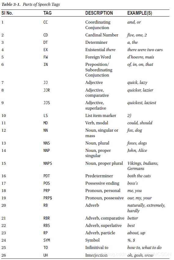
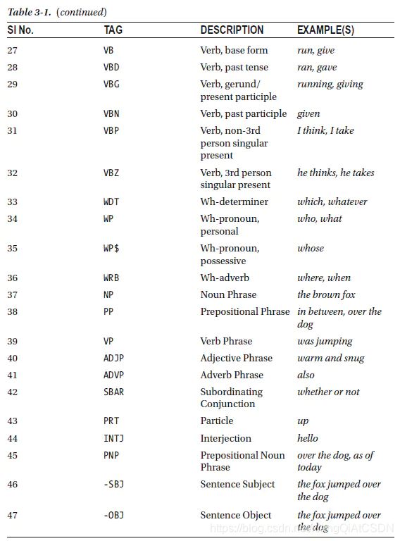
关于上述词性的说明:
示例的Python代码
from nltk import word_tokenize, pos_tag
from nltk.corpus import wordnet
from nltk.stem import WordNetLemmatizer

# 获取单词的词性
def get_wordnet_pos(tag):
    if tag.startswith('J'):
        return wordnet.ADJ
    elif tag.startswith('V'):
        return wordnet.VERB
    elif tag.startswith('N'):
        return wordnet.NOUN
    elif tag.startswith('R'):
        return wordnet.ADV
    else:
        return None

sentence = 'football is a family of team sports that involve, to varying degrees, kicking a ball to score a goal.'
tokens = word_tokenize(sentence)  # 分词
tagged_sent = pos_tag(tokens)     # 获取单词词性

wnl = WordNetLemmatizer()
lemmas_sent = []
for tag in tagged_sent:
    wordnet_pos = get_wordnet_pos(tag[1]) or wordnet.NOUN
    lemmas_sent.append(wnl.lemmatize(tag[0], pos=wordnet_pos)) # 词形还原

print(lemmas_sent)
输出结果如下:
['football', 'be', 'a', 'family', 'of', 'team', 'sport', 'that', 'involve', ',', 'to', 'vary', 'degree', ',', 'kick', 'a', 'ball', 'to', 'score', 'a', 'goal', '.']
这就是对句子中的单词进行词形还原后的结果。
4. 命名实体识别(NER)
什么是NER
命名实体识别(Named Entity Recognition,简称NER)是信息提取、问答系统、句法分析、机器翻译等应用领域的重要基础工具,在自然语言处理技术走向实用化的过程中占有重要地位。一般来说,命名实体识别的任务就是识别出待处理文本中三大类(实体类、时间类和数字类)、七小类(人名、机构名、地名、时间、日期、货币和百分比)命名实体。
举个简单的例子,在句子“小明早上8点去学校上课。”中,对其进行命名实体识别,应该能提取信息
人名:小明,时间:早上8点,地点:学校。
我们将会介绍几个工具用来进行命名实体识别,后续有机会的话,我们将会尝试着用HMM、CRF或深度学习来实现命名实体识别。
分类细节与工具
首先我们来看一下NLTK和Stanford NLP中对命名实体识别的分类,如下图:
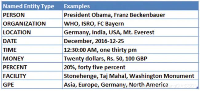
在上图中,LOCATION和GPE有重合。GPE通常表示地理—政治条目,比如城市,州,国家,洲等。LOCATION除了上述内容外,还能表示名山大川等。FACILITY通常表示知名的纪念碑或人工制品等。
下面介绍两个工具来进行NER的任务:NLTK和Stanford NLP。
首先是NLTK,我们的示例文档(介绍FIFA,来源于维基百科)如下:
FIFA was founded in 1904 to oversee international competition among the national associations of Belgium,
Denmark, France, Germany, the Netherlands, Spain, Sweden, and Switzerland. Headquartered in Zürich, its
membership now comprises 211 national associations. Member countries must each also be members of one of
the six regional confederations into which the world is divided: Africa, Asia, Europe, North & Central America
and the Caribbean, Oceania, and South America.
使用nltk实现NER
import re
import pandas as pd
import nltk

def parse_document(document):
   document = re.sub('\n', ' ', document)
   if isinstance(document, str):
       document = document
   else:
       raise ValueError('Document is not string!')
   document = document.strip()
   sentences = nltk.sent_tokenize(document)
   sentences = [sentence.strip() for sentence in sentences]
   return sentences

# sample document
text = """
FIFA was founded in 1904 to oversee international competition among the national associations of Belgium,
Denmark, France, Germany, the Netherlands, Spain, Sweden, and Switzerland. Headquartered in Zürich, its
membership now comprises 211 national associations. Member countries must each also be members of one of
the six regional confederations into which the world is divided: Africa, Asia, Europe, North & Central America
and the Caribbean, Oceania, and South America.
"""

# tokenize sentences
sentences = parse_document(text)
tokenized_sentences = [nltk.word_tokenize(sentence) for sentence in sentences]
# tag sentences and use nltk's Named Entity Chunker
tagged_sentences = [nltk.pos_tag(sentence) for sentence in tokenized_sentences]
ne_chunked_sents = [nltk.ne_chunk(tagged) for tagged in tagged_sentences]
# extract all named entities
named_entities = []
for ne_tagged_sentence in ne_chunked_sents:
   for tagged_tree in ne_tagged_sentence:
       # extract only chunks having NE labels
       if hasattr(tagged_tree, 'label'):
           entity_name = ' '.join(c[0] for c in tagged_tree.leaves()) #get NE name
           entity_type = tagged_tree.label() # get NE category
           named_entities.append((entity_name, entity_type))
           # get unique named entities
           named_entities = list(set(named_entities))

# store named entities in a data frame
entity_frame = pd.DataFrame(named_entities, columns=['Entity Name', 'Entity Type'])
# display results
print(entity_frame)
输出结果:
        Entity Name   Entity Type
0              FIFA  ORGANIZATION
1   Central America  ORGANIZATION
2           Belgium           GPE
3         Caribbean      LOCATION
4              Asia           GPE
5            France           GPE
6           Oceania           GPE
7           Germany           GPE
8     South America           GPE
9           Denmark           GPE
10           Zürich           GPE
11           Africa        PERSON
12           Sweden           GPE
13      Netherlands           GPE
14            Spain           GPE
15      Switzerland           GPE
16            North           GPE
17           Europe           GPE
可以看到,NLTK中的NER任务大体上完成得还是不错的,能够识别FIFA为组织(ORGANIZATION),Belgium,Asia为GPE, 但是也有一些不太如人意的地方,比如,它将Central America识别为ORGANIZATION,而实际上它应该为GPE;将Africa识别为PERSON,实际上应该为GPE。
实现Stanford NER
接下来,我们尝试着用Stanford NLP工具。关于该工具,我们主要使用Stanford NER 标注工具。在使用这个工具之前,你需要在自己的电脑上安装Java(一般是JDK),并将Java添加到系统路径中,同时下载英语NER的文件包:stanford-ner-2018-10-16.zip(大小为172MB),下载地址为:https://nlp.stanford.edu/software/CRF-NER.shtml。以我的电脑为例,Java所在的路径为:C:\Program Files\Java\jdk1.8.0_161\bin\java.exe, 下载Stanford NER的zip文件解压后的文件夹的路径为:E://stanford-ner-2018-10-16,在classifer文件夹中有如下文件:
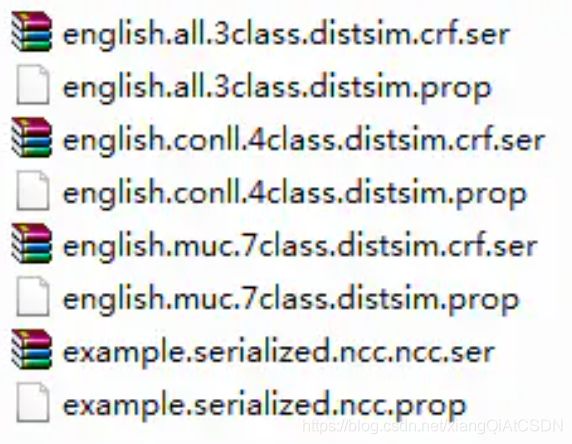
它们的含义为:
3 class: Location, Person, Organization
4 class: Location, Person, Organization, Misc
7 class: Location, Person, Organization, Money, Percent, Date, Time
实现代码如下:
import re
from nltk.tag import StanfordNERTagger
import os
import pandas as pd
import nltk

def parse_document(document):
   document = re.sub('\n', ' ', document)
   if isinstance(document, str):
       document = document
   else:
       raise ValueError('Document is not string!')
   document = document.strip()
   sentences = nltk.sent_tokenize(document)
   sentences = [sentence.strip() for sentence in sentences]
   return sentences

# sample document
text = """
FIFA was founded in 1904 to oversee international competition among the national associations of Belgium,
Denmark, France, Germany, the Netherlands, Spain, Sweden, and Switzerland. Headquartered in Zürich, its
membership now comprises 211 national associations. Member countries must each also be members of one of
the six regional confederations into which the world is divided: Africa, Asia, Europe, North & Central America
and the Caribbean, Oceania, and South America.
"""

sentences = parse_document(text)
tokenized_sentences = [nltk.word_tokenize(sentence) for sentence in sentences]

# set java path in environment variables
java_path = r'C:\Program Files\Java\jdk1.8.0_161\bin\java.exe'
os.environ['JAVAHOME'] = java_path
# load stanford NER
sn = StanfordNERTagger('E://stanford-ner-2018-10-16/classifiers/english.muc.7class.distsim.crf.ser.gz',
                       path_to_jar='E://stanford-ner-2018-10-16/stanford-ner.jar')

# tag sentences
ne_annotated_sentences = [sn.tag(sent) for sent in tokenized_sentences]
# extract named entities
named_entities = []
for sentence in ne_annotated_sentences:
   temp_entity_name = ''
   temp_named_entity = None
   for term, tag in sentence:
       # get terms with NE tags
       if tag != 'O':
           temp_entity_name = ' '.join([temp_entity_name, term]).strip() #get NE name
           temp_named_entity = (temp_entity_name, tag) # get NE and its category
       else:
           if temp_named_entity:
               named_entities.append(temp_named_entity)
               temp_entity_name = ''
               temp_named_entity = None

# get unique named entities
named_entities = list(set(named_entities))
# store named entities in a data frame
entity_frame = pd.DataFrame(named_entities, columns=['Entity Name', 'Entity Type'])
# display results
print(entity_frame)
输出结果如下:
                Entity Name   Entity Type
0                      1904          DATE
1                   Denmark      LOCATION
2                     Spain      LOCATION
3   North & Central America  ORGANIZATION
4             South America      LOCATION
5                   Belgium      LOCATION
6                    Zürich      LOCATION
7           the Netherlands      LOCATION
8                    France      LOCATION
9                 Caribbean      LOCATION
10                   Sweden      LOCATION
11                  Oceania      LOCATION
12                     Asia      LOCATION
13                     FIFA  ORGANIZATION
14                   Europe      LOCATION
15                   Africa      LOCATION
16              Switzerland      LOCATION
17                  Germany      LOCATION
可以看到,在Stanford NER的帮助下,NER的实现效果较好,将Africa识别为LOCATION,将1904识别为时间(这在NLTK中没有识别出来),但还是对North & Central America识别有误,将其识别为ORGANIZATION。
值得注意的是,并不是说Stanford NER一定会比NLTK NER的效果好,两者针对的对象,预料,算法可能有差异,因此,需要根据自己的需求决定使用什么工具。