Logistic Regression逻辑线性回归（基于diabetes数据集）

目录

介绍： 

1、Confusion Matrix：

2、ROC（Receiver Operating Characteristic） 

 一、数据处理

二、建模

三、 confusion_matrix

四、 ROC（Receiver Operating Characteristic）

介绍： 

Logistic Regression（逻辑回归）是一种用于解决分类问题的统计学习方法。它是线性回归的一种改进，主要用于处理二分类问题，也可以通过修改算法来处理多分类问题。

Logistic Regression的主要思想是通过线性回归模型的线性组合，将其映射到一个特定的函数（称为sigmoid函数）的输出范围内，从而将输入数据映射为一个概率值。sigmoid函数的输出范围为0到1之间，表示某个样本属于某个类别的概率。

Logistic Regression的训练过程是通过最大似然估计来求解模型参数。通常使用梯度下降等优化算法来最小化损失函数。在预测阶段，通过计算模型的输出概率值，并根据设定的阈值进行分类决策。

Logistic Regression具有简单、易于解释的优点，可以用于解决许多实际应用中的分类问题，如垃圾邮件过滤、信用风险评估、医学诊断等。然而，它也有一些限制，例如容易受到特征间相关性的影响，对于非线性分类问题的性能可能较差。

1、Confusion Matrix：

混淆矩阵（Confusion Matrix）是一种用于评估分类模型结果的方法。它以矩阵的形式展示了模型对样本的分类情况。

混淆矩阵的表格中有四个不同的结果：

真正类（True Positive，TP）：模型正确地将正类样本分类为正类。
真负类（True Negative，TN）：模型正确地将负类样本分类为负类。
假正类（False Positive，FP）：模型错误地将负类样本分类为正类。
假负类（False Negative，FN）：模型错误地将正类样本分类为负类。

混淆矩阵通过统计分类结果的各个类别，可以计算出许多分类模型的性能指标，如准确率、召回率、精确率和F1-Score等。通过分析混淆矩阵，可以帮助我们对分类模型的性能进行评估和改进。

 

2、ROC（Receiver Operating Characteristic） 

ROC（Receiver Operating Characteristic）是一种用于评估分类模型性能的曲线，常用于二分类问题。在Logistic回归中，ROC曲线是通过改变分类模型的阈值而绘制出来的。

ROC曲线的横坐标是分类模型的假阳性率（False Positive Rate，FPR），纵坐标是分类模型的真阳性率（True Positive Rate，TPR），也就是分类模型的灵敏度（Sensitivity）。

在Logistic回归中，模型对样本进行概率预测，然后通过设定一个阈值将概率转化为分类标签。阈值越低，模型将更多的样本预测为阳性，从而会增加假阳性的数量，降低真阳性的数量；阈值越高，模型将更少的样本预测为阳性，从而会降低假阳性的数量，增加真阳性的数量。ROC曲线通过改变这个阈值，分别计算不同阈值下的FPR和TPR，然后将这些点连接起来得到。

ROC曲线越靠近左上角，表示分类模型的性能越好，因为这意味着在较低的假阳性率下能获得较高的真阳性率。ROC曲线下的面积（Area Under Curve，AUC）也是评估分类模型性能的重要指标。AUC的取值范围在0.5到1之间，越接近1表示模型性能越好。

 一、数据处理

import numpy as np
import pandas as pd
import matplotlib.pyplot as plt
from sklearn.linear_model import LogisticRegression#逻辑线性回归，结果是二分类
from sklearn.model_selection import train_test_split
from sklearn.metrics import confusion_matrix

data=pd.read_csv("diabetes.csv")

X=data.iloc[:,:-1]
y=data.iloc[:,-1]

data：

plt.rcParams['font.sans-serif']=['SimHei']#用来正常显示中文标签
plt.rcParams['axes.unicode_minus']=False#用来正常显示负号

plt.plot(X,y,'o')
plt.title('logistic regression 二分类 Binary classification')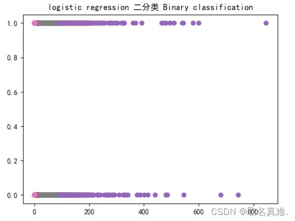

二、建模

X_train,X_test,y_train,y_test=train_test_split(X,y,test_size=0.3,random_state=0)#测试集占百分之三十，random_state=0随机抽取数据集里的成为测试集是一样的

X_train.shape
#结果：(537, 8)

X_test.shape
#结果：(231, 8)

logregression = LogisticRegression()
logregression.fit(X_train,y_train)#训练集赋给模型

y_predict=logregression.predict(X_test)#预测值
'''结果：
array([1, 0, 0, 1, 0, 0, 1, 1, 0, 0, 1, 1, 0, 0, 0, 0, 1, 0, 0, 0, 1, 0,
       0, 0, 0, 0, 0, 1, 0, 0, 0, 0, 0, 0, 0, 1, 0, 0, 0, 1, 0, 0, 0, 1,
       1, 0, 0, 0, 0, 0, 0, 0, 1, 1, 0, 0, 0, 1, 0, 0, 1, 0, 0, 1, 1, 1,
       1, 0, 0, 0, 0, 0, 0, 1, 1, 0, 0, 1, 0, 0, 0, 0, 0, 0, 0, 0, 0, 0,
       1, 0, 0, 0, 0, 0, 1, 0, 0, 1, 1, 0, 0, 0, 0, 0, 1, 0, 0, 0, 0, 1,
       0, 0, 1, 0, 1, 1, 0, 1, 0, 1, 0, 0, 0, 0, 0, 0, 0, 0, 0, 0, 0, 0,
       0, 1, 0, 0, 0, 0, 1, 0, 0, 1, 0, 0, 0, 0, 0, 0, 0, 0, 0, 1, 0, 0,
       1, 0, 1, 0, 0, 1, 1, 1, 0, 0, 1, 0, 0, 0, 0, 0, 0, 0, 0, 0, 1, 0,
       0, 0, 0, 0, 0, 1, 0, 1, 0, 0, 1, 0, 0, 0, 0, 0, 0, 0, 0, 1, 1, 0,
       0, 0, 0, 0, 0, 0, 0, 0, 0, 0, 0, 0, 0, 0, 0, 0, 0, 0, 0, 0, 1, 0,
       0, 0, 0, 1, 1, 1, 0, 0, 0, 0, 0], dtype=int64)
'''

logregression.score(X_test,y_test)#模型的精确率
#结果：0.7792207792207793

三、 confusion_matrix

confusion_matrix(y_test,y_predict)
#结果：array([[141,  16],
#             [ 35,  39]], dtype=int64)

from sklearn.metrics import classification_report
print(classification_report(y_test,y_predict))
#support的0=141+16，support的1=上面35+39
#presion的0 表示预测0的准确率， pression的1 表示预测1的准确率
#recall召回率 reacall的1=141/（141+35） recall的0=39/（39+35）
'''结果：
                precision    recall  f1-score   support

           0       0.80      0.90      0.85       157
           1       0.71      0.53      0.60        74

    accuracy                           0.78       231
   macro avg       0.76      0.71      0.73       231
weighted avg       0.77      0.78      0.77       231
'''

print(logregression.coef_)#八项参数
'''结果：
[[ 0.0852812   0.03447238 -0.01082113  0.00636549 -0.0013322   0.08852981
   0.73271467  0.02415028]]
'''

print(logregression.intercept_)#y轴切入
#结果：[-8.60539142]

四、 ROC（Receiver Operating Characteristic）

from sklearn.metrics import roc_auc_score
from sklearn.metrics import roc_curve
logrocauc=roc_auc_score(y_test,logregression.predict(X_test))
fpr,tpr,thresholds=roc_curve(y_test,logregression.predict_proba(X_test)[:,1])
plt.figure()
plt.plot(fpr,tpr,label='Logistic Regression (area=%0.3f)'%logrocauc)
plt.plot([0,1],[0,1],'r--')
plt.xlim([0.0,1.05])
plt.ylim([0.0,1.05])
plt.xlabel('False Positive Rate')
plt.ylabel('True Positive Rate')
plt.title('Receiver operating characteristic')
plt.legend(loc='lower right')