DSS (Dispersion Shrinkage for Sequencing data),为基于高通量测序数据的差异分析而设计的Bioconductor包。主要应用于BS-seq(亚硫酸氢盐测序)中计算不同组别间差异甲基化位点(DML)和差异甲基化区域(DMR)即Call DML or DMR。
Bisulfite Sequencing (BS-Seq)上游测序数据可以得到甲基化位点的信息,而后续DML以及DMR的确定以及可视化就需要DSS包。
DSS包的使用主要包括:输入文件的准备 --> 利用DMLtest函数call DML --> 利用callDML函数Call DML --> 利用callDMR函数Call DMR --> 利用showOneDMR函数对DMRs可视化
1.输入文件准备
DSS包要求输入文件数据的格式如下:
每一行代表一个CpG site
Below shows an example of a small part of such a file:

chr pos N X
chr18 3014904 26 2
chr18 3031032 33 12
chr18 3031044 33 13
chr18 3031065 48 24
- 第一列为染色体
- 第二列为位置
- 第三列为total reads
- 第四列为甲基化的reads
拿到上游比对结果后需要把结果文件*.bismark.cov.gz改成DSS包所要求的样子,使用Linux或者R进行简单的处理及可得到input文件。
2. 计算不同组别间差异甲基化位点和区域—Call DML or DMR
DML:甲基化差异位点;DMR:甲基化差异区域
使用DSS包自带的数据演示如何计算不同组别间差异甲基化位点和区域
2.1 载入DSS和bsseq包构建BSobj对象
library(DSS)
require(bsseq)
path <- file.path(system.file(package="DSS"), "extdata")
dat1.1 <- read.table(file.path(path, "cond1_1.txt"), header=TRUE)
dat1.2 <- read.table(file.path(path, "cond1_2.txt"), header=TRUE)
dat2.1 <- read.table(file.path(path, "cond2_1.txt"), header=TRUE)
dat2.2 <- read.table(file.path(path, "cond2_2.txt"), header=TRUE)
BSobj <- makeBSseqData( list(dat1.1, dat1.2, dat2.1, dat2.2),
                        c("C1","C2", "N1", "N2") )[1:1000,]

> BSobj
An object of type 'BSseq' with
1000 methylation loci
4 samples
has not been smoothed
All assays are in-memory
2.2 利用DMLtest函数call DML
DML:甲基化差异位点;DMR:甲基化差异区域
DMLtest函数主要包括以下步骤:
- 计算所有CpG位点的平均甲基化水平;
- 计算每个CpG位点的分散度dispersions;
- 进行沃尔德检验 conduct Wald test
在第一步过程中,我们可以选择是否smoothing处理甲基化水平。当测序结果中CpG 位点特别密集时(比如:whole-genome BS-seq得到的数据)smoothing处理可以以更简洁直接的方式帮助估算平均甲基化水平;当CpG 位点比较稀疏时(比如:RRBS or hydroxyl-methylation得到的数据)则不需要smoothing处理。
Call DML时不经过smoothing处理:
# To perform DML test without smoothing, do:
dmlTest <- DMLtest(BSobj, group1=c("C1", "C2"), group2=c("N1", "N2"))

> head(dmlTest)
    chr     pos       mu1       mu2        diff    diff.se       stat        phi1       phi2       pval       fdr
1 chr18 3014904 0.3817233 0.4624549 -0.08073162 0.24997034 -0.3229648 0.300542998 0.01706260 0.74672190 0.9985094
2 chr18 3031032 0.3380579 0.1417008  0.19635711 0.11086362  1.7711592 0.008911745 0.04783892 0.07653423 0.6792127
3 chr18 3031044 0.3432172 0.3298853  0.01333190 0.12203116  0.1092500 0.010409029 0.01994821 0.91300423 0.9985094
4 chr18 3031065 0.4369377 0.3649218  0.07201587 0.10099395  0.7130711 0.010320888 0.01603200 0.47580174 0.9985094
5 chr18 3031069 0.2933572 0.5387464 -0.24538920 0.13178800 -1.8619996 0.012537553 0.02320887 0.06260315 0.6158797
6 chr18 3031082 0.3526311 0.3905718 -0.03794068 0.07847999 -0.4834440 0.007665696 0.01145531 0.62878051 0.9985094
Call DML时经过smoothing处理代码:
# To perform statistical test for DML with smoothing, do:
dmlTest.sm <- DMLtest(BSobj, group1=c("C1", "C2"), group2=c("N1", "N2"), smoothing=TRUE)

> head(dmlTest.sm)
    chr     pos       mu1       mu2        diff    diff.se       stat       phi1       phi2      pval       fdr
1 chr18 3014904 0.3693669 0.4566563 -0.08728939 0.29967322 -0.2912819 0.30054300 0.01706260 0.7708357 0.9656515
2 chr18 3031032 0.3433882 0.3679732 -0.02458503 0.03970109 -0.6192533 0.03177894 0.28323422 0.5357495 0.8639036
3 chr18 3031044 0.3412867 0.3678807 -0.02659404 0.04032823 -0.6594397 0.02536938 0.02080295 0.5096134 0.8596522
4 chr18 3031065 0.3358830 0.3511983 -0.01531533 0.04799161 -0.3191252 0.01123412 0.01621926 0.7496316 0.9652417
5 chr18 3031069 0.3358830 0.3511983 -0.01531533 0.03205500 -0.4777830 0.02832889 0.05857316 0.6328047 0.8968029
6 chr18 3031082 0.3358830 0.3511983 -0.01531533 0.05846593 -0.2619531 0.01682981 0.01368466 0.7933576 0.9745116
2.3 利用callDML函数call DML
使用callDML函数call DML,结果可以按显著性排序:
dmls <- callDML(dmlTest, p.threshold=0.001)
> head(dmls)
      chr     pos        mu1       mu2       diff    diff.se      stat        phi1       phi2         pval          fdr
450 chr18 3976129 0.01027497 0.9390339 -0.9287590 0.06544340 -14.19179 0.052591567 0.02428826 1.029974e-45 2.499403e-43
451 chr18 3976138 0.01027497 0.9390339 -0.9287590 0.06544340 -14.19179 0.052591567 0.02428826 1.029974e-45 2.499403e-43
638 chr18 4431501 0.01331553 0.9430566 -0.9297411 0.09273779 -10.02548 0.053172411 0.07746835 1.177826e-23 1.429096e-21
639 chr18 4431511 0.01327049 0.9430566 -0.9297862 0.09270080 -10.02997 0.053121697 0.07746835 1.125518e-23 1.429096e-21
710 chr18 4564237 0.91454619 0.0119300  0.9026162 0.05260037  17.15988 0.009528898 0.04942849 5.302004e-66 3.859859e-63
782 chr18 4657576 0.98257334 0.0678355  0.9147378 0.06815000  13.42242 0.010424723 0.06755651 4.468885e-41 8.133371e-39
    postprob.overThreshold
450                      1
451                      1
638                      1
639                      1
710                      1
782                      1
默认情况下,计算基于零假设,即默认甲基化水平的差异为0。当然,我们可以指定差异的阈值,只有差异大于阈值(0.1)的才会被call出来:
# To detect loci with difference greater than 0.1, do:
> dmls2 <- callDML(dmlTest, delta=0.1, p.threshold=0.001)
> head(dmls2)
      chr     pos        mu1       mu2       diff    diff.se      stat        phi1       phi2         pval
450 chr18 3976129 0.01027497 0.9390339 -0.9287590 0.06544340 -14.19179 0.052591567 0.02428826 1.029974e-45
451 chr18 3976138 0.01027497 0.9390339 -0.9287590 0.06544340 -14.19179 0.052591567 0.02428826 1.029974e-45
638 chr18 4431501 0.01331553 0.9430566 -0.9297411 0.09273779 -10.02548 0.053172411 0.07746835 1.177826e-23
639 chr18 4431511 0.01327049 0.9430566 -0.9297862 0.09270080 -10.02997 0.053121697 0.07746835 1.125518e-23
710 chr18 4564237 0.91454619 0.0119300  0.9026162 0.05260037  17.15988 0.009528898 0.04942849 5.302004e-66
782 chr18 4657576 0.98257334 0.0678355  0.9147378 0.06815000  13.42242 0.010424723 0.06755651 4.468885e-41
             fdr postprob.overThreshold
450 2.499403e-43                      1
451 2.499403e-43                      1
638 1.429096e-21                      1
639 1.429096e-21                      1
710 3.859859e-63                      1
782 8.133371e-39                      1
2.4 利用callDMR函数Call DMR
DML:甲基化差异位点;DMR:甲基化差异区域
甲基化差异区域检测也是基于差异位点的结果,同样使用callDML函数。当不同组别间CpG位点区域具有显著的统计学差异时这段差异区域被定义为DMRs。
# Call DMR by using callDMR function
##Regions with many statistically significant CpG sites are identified as DMRs.
dmrs <- callDMR(dmlTest, p.threshold=0.01)
> head(dmrs)
     chr   start     end length nCG meanMethy1 meanMethy2 diff.Methy areaStat
27 chr18 4657576 4657639     64   4   0.506453   0.318348   0.188105 14.34236
同理,这里我们也可以使用delta参数以及调整p.threshold指定差异的阈值:
# To detect regions with difference greater than 0.1, do:
dmrs2 <- callDMR(dmlTest, delta=0.1, p.threshold=0.05)
> head(dmrs2)
     chr   start     end length nCG meanMethy1 meanMethy2 diff.Methy areaStat
31 chr18 4657576 4657639     64   4  0.5064530  0.3183480   0.188105 14.34236
19 chr18 4222533 4222608     76   4  0.7880276  0.3614195   0.426608 12.91667
这里我们需要注意,选择一个合理的阈值来定义DMRs是非常困难的,所以建议尝试不同的阈值,以获得满意的结果。
2.5 可视化
使用showOneDMR函数可视化甲基化差异区域DML,该函数不仅可以绘制甲基化所占百分比还可以绘制每个CpG位点的覆盖深度。
showOneDMR(dmrs[1,], BSobj)
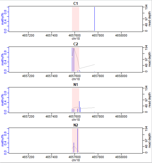
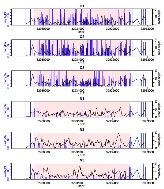
我们的示例数据来自RRBS实验结果,所以甲基化差异区域DML很短。一般whole-genome BS-seq数据中DML会长一些:
代码纯享版:
# 1. Load in library. Read in text files and create an object of BSseq class
library(DSS)
require(bsseq)
path <- file.path(system.file(package="DSS"), "extdata")
dat1.1 <- read.table(file.path(path, "cond1_1.txt"), header=TRUE)
dat1.2 <- read.table(file.path(path, "cond1_2.txt"), header=TRUE)
dat2.1 <- read.table(file.path(path, "cond2_1.txt"), header=TRUE)
dat2.2 <- read.table(file.path(path, "cond2_2.txt"), header=TRUE)
BSobj <- makeBSseqData( list(dat1.1, dat1.2, dat2.1, dat2.2),
                        c("C1","C2", "N1", "N2") )[1:1000,]
BSobj

# 2.Perform statistical test for DML by calling DMLtest function.
## To perform DML test without smoothing, do:
dmlTest <- DMLtest(BSobj, group1=c("C1", "C2"), group2=c("N1", "N2"))
head(dmlTest)
## To perform statistical test for DML with smoothing, do:
dmlTest.sm <- DMLtest(BSobj, group1=c("C1", "C2"), group2=c("N1", "N2"), smoothing=TRUE)
head(dmlTest.sm)

# 3.Call DML by using callDML function. The results DMLs are sorted by the significance.
dmls <- callDML(dmlTest, p.threshold=0.001)
head(dmls)
##To detect loci with difference greater than 0.1, do:
dmls2 <- callDML(dmlTest, delta=0.1, p.threshold=0.001)
head(dmls2)

# 4.Call DMR by using callDML function
##Regions with many statistically significant CpG sites are identified as DMRs.
dmrs <- callDMR(dmlTest, p.threshold=0.01)
head(dmrs)
##To detect regions with difference greater than 0.1, do:
dmrs2 <- callDMR(dmlTest, delta=0.1, p.threshold=0.05)
head(dmrs2)

# 5.The DMRs can be visualized using showOneDMR function
showOneDMR(dmrs[1,], BSobj)