qlib因子分析之alphalens源码解读
百天计划第33篇,不知不觉一个多月。
"N阶行动"计划第2阶,这一阶就告诉自己要坚持,差不多可以挺过去。
坚持并不容易,早上起来心情有起伏。
投资说简单非常简单,就是低卖高卖;往难里说可能扯到宇宙星辰,人性善恶。
在量化人的眼中,一切都是因子。
技术面是因子,基本面也是因子。
有点像体验里验血、尿,B超等,给出一系列量化指标,再结合你的表述,症状,有经验的医生就可以给出结果。
当然总有很多信息是难以量化的,人是一个复杂系统。
股票也一样,所以才需要医生的存在。
量化投资本质上就是“找因子”,技术分析里可以量化的部分都是因子,因子进入模型不是hard-code的,而是以概率的形式,这就存在可以学习和优化的空间。
传统动量模型,比如20日动量>0.02就买入,小于0就卖出,和MACD>0一样,在大牛市非常好,震荡市让你怀疑人生,关键是你不知道当前是什么趋势。拉开了周期,这些因子都是alpha。
01 因子数据准备
alphalens的代码量不大,一共就4个文件:
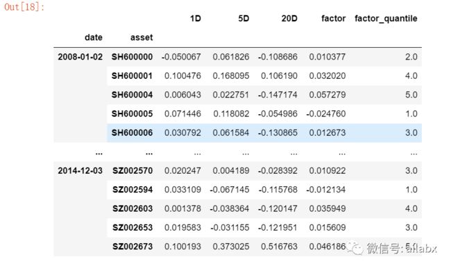
get_clean_factor_and_forward_returns,在utils.py里。
这个函数返回如下格式的数据,它基于的输入:
因子值,这个还在下表中未动,但给因子分5层(quantile)。
基于价格prices,计算出未来1天(D),5天和20天的收益率。
具体想计算多少天都行,用periods=(1,5,20)来设置即可。
改成periods=(1,5,10,15,20),其实就是计算N天的预期收益率。
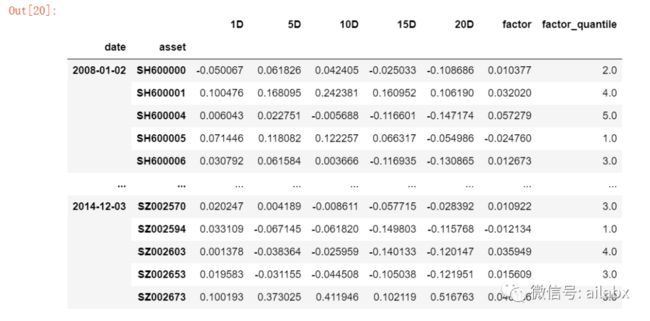
核心代码如下:
forward_returns = compute_forward_returns(
    factor,
    prices,
    periods,
    filter_zscore,
    cumulative_returns,
)

factor_data = get_clean_factor(factor, forward_returns, groupby=groupby,
                               groupby_labels=groupby_labels,
                               quantiles=quantiles, bins=bins,
                               binning_by_group=binning_by_group,
                               max_loss=max_loss, zero_aware=zero_aware)
compute_forward_returns就是计算“预期收益率”。
使用dataframe的 N期“变化率”,就是收益率。
for period in sorted(periods):
    if cumulative_returns:
        returns = prices.pct_change(period)
然后使用pandas的qcut函数,把因子分成5等分。
def quantile_calc(x, _quantiles, _bins, _zero_aware, _no_raise):
    try:
        if _quantiles is not None and _bins is None and not _zero_aware:
            return pd.qcut(x, _quantiles, labels=False) + 1
        elif _quantiles is not None and _bins is None and _zero_aware:
            pos_quantiles = pd.qcut(x[x >= 0], _quantiles // 2,
                                    labels=False) + _quantiles // 2 + 1
            neg_quantiles = pd.qcut(x[x < 0], _quantiles // 2,
                                    labels=False) + 1
            return pd.concat([pos_quantiles, neg_quantiles]).sort_index()
        elif _bins is not None and _quantiles is None and not _zero_aware:
            return pd.cut(x, _bins, labels=False) + 1
        elif _bins is not None and _quantiles is None and _zero_aware:
            pos_bins = pd.cut(x[x >= 0], _bins // 2,
                              labels=False) + _bins // 2 + 1
            neg_bins = pd.cut(x[x < 0], _bins // 2,
                              labels=False) + 1
            return pd.concat([pos_bins, neg_bins]).sort_index()
    except Exception as e:
        if _no_raise:
            return pd.Series(index=x.index)
        raise e
02 因子分析
create_full_tear_sheet这个函数是总体分析入口。
一共做了四件事:
统计分位表:
plotting.plot_quantile_statistics_table(factor_data)
一共就两行代码:
quantile_stats = factor_data.groupby('factor_quantile') \
    .agg(['min', 'max', 'mean', 'std', 'count'])['factor']
quantile_stats['count %'] = quantile_stats['count'] \
    / quantile_stats['count'].sum() * 100.
就是因子值,按分位分组后,计算“最小值min”,"最大值max",“均值mean”,"标准差std"。大约每个分位占20%,符合预期。
这里可能会引发一个困惑:第一分位的max不应该 <= 第二分位的min嘛 ,怎么有这么多重叠?——按天分的,每天都分5段,总体来看,就会有区间重叠。
第二步:收益分析:
create_returns_tear_sheet(
    factor_data, long_short, group_neutral, by_group, set_context=False
)
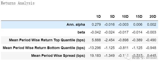
等权买入5个分位的股票后,可以计算各周期的收益率。
平均收益与分位收益之间的回归分析:
universe_ret = factor_data.groupby(level='date')[
    utils.get_forward_returns_columns(factor_data.columns)] \
    .mean().loc[returns.index]
使用线性回归OLS:
alpha_beta = pd.DataFrame()
for period in returns.columns.values:
    x = universe_ret[period].values
    y = returns[period].values
x = add_constant(x)
  reg_fit = OLS(y, x).fit()
    try:
        alpha, beta = reg_fit.params
计算出alpha和beta。
收益分析看起来有点类似“回测”,按因子高低买卖,看回测结果——结果都不错,但似乎没什么用,关键还看“信息分析”。
第三步:信息分析:
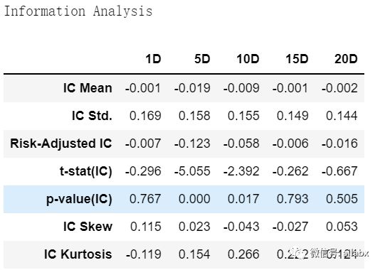
def src_ic(group):
    f = group['factor']
    _ic = group[utils.get_forward_returns_columns(factor_data.columns)] \
        .apply(lambda x: stats.spearmanr(x, f)[0])
    return _ic
IC值就是相关系数,这个之前文章说过了。
相关系数都是负的,且绝对值小于0.05,就是不显著,或者说这个因子没啥用。
第四:换手率分析:
create_turnover_tear_sheet(factor_data, set_context=False)
小结:
基本把目前传统的因子分析说完了,展开代码来看,没有什么神秘的,就是基础统计分析和线性回归。
单因子分析的逻辑是这样的,把因子从小到大分成5组,每天等权买这组,看period=1,5,10...之后的收益率情况。这是收益分析;把因子值直接与收益序列做相关性分析,得到IC值。最后交易会有换手率的问题。
最近文章:
基于alphalens对qlib的alpha158做单因子分析
人生B计划,不确定时代的应对之道
持续行动——从想到到做到
飞狐,科技公司CTO,用AI技术做量化投资;以投资视角观历史,解时事;专注个人成长与财富自由。