cs231n作业 assignment 1 q1 q2 q3
文章目录
- 前言 嫌啰嗦直接看源码
- 作业一内容
- Q1 knn分类器
-
- compute_distance_two_loops
-
- 题面
- 解析
- 代码
- 输出
- Inline Question 1
-
- 题面
- 解答
- predict_labels
-
- 题面
- 解析
- 代码
- 结果
- Inline Question 2
-
- 题面
- 解答
- compute_distances_one_loop
-
- 题面
- 解答
- 代码
- compute_distances_no_loops
-
- 题面
- 解析
- 代码
- Cross-validation
-
- 题面
- 代码
- 解析
- 输出
- 最后
- Q2 Training a Support Vector Machine
-
- svm_loss_naive
-
- 题面
- 解析
- 代码
- svm_loss_vectorized (loss)
-
- 题面
- 解析
- 代码
- 输出
- svm_loss_vectorized (gradient)
-
- 题面
- 解析
- 代码
- 输出
- LinearClassifier.train
-
- 题面
- 解析
- 代码
- 输出
- predict
-
- 题面
- 代码
- 输出
- 找到最好的hypeparameter
-
- 题面
- 代码
- 输出
- 最后输出最后的结果
- Q3 softmax
-
- softmax 讲解与梯度推导
- softmax_loss_naive
-
- 题面
- 解析
- 代码
- 结果
- softmax_loss_vectorized
-
- 题面
- 解析
- 代码
- 找到最好的hypeparameter
-
- 题面
- 解析
- 代码
- 输出
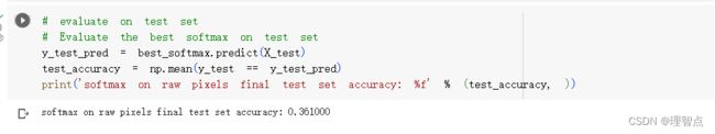
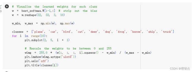
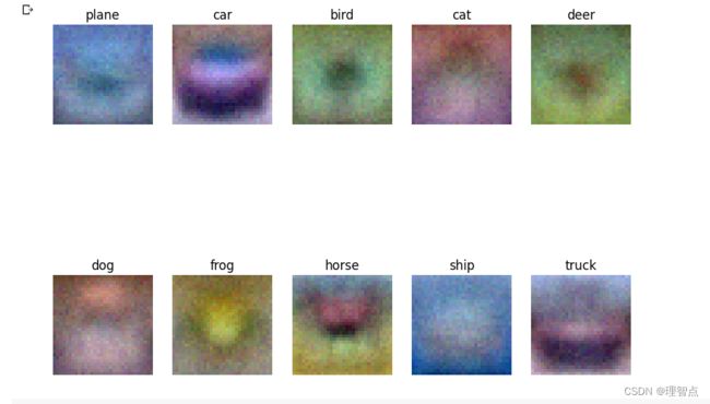
- 最后的结果
前言 嫌啰嗦直接看源码
请先看课程,作业地址。
有两种做作业的方法,一种是在google Colab上做 (需魔法),另一种就是下载到本地,但是我懒得在本地配置环境,太麻烦了,还得修改一些基础代码,我就直接在google colab上做了
google colab 配置环境只需要跟着教程走就好了
作业一内容
同时配置colab环境的教程也在这个页面https://cs231n.github.io/assignments2023/assignment1/#setup
Q1 knn分类器
compute_distance_two_loops
题面
解析
打开文件可以看到这里
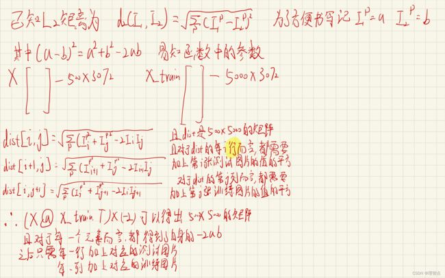
让我们计算X_test 和 X_train之间图像之间的l2距离,第i个X_test的图像和第J个X_train的图像的距离存放在dists[i,j]中
L1距离和L2距离的解释

有了上面那个公式,我们实现起来就很简单了
用np.sqrt(np.sum(np.power()))的方法就好了,这个主要是考察对np的几个库函数的熟悉程度
但是因为这个方法的时间复杂的大概是50005003072,所以我跑了大概五分钟!!
代码
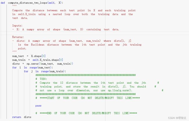
    def compute_distances_two_loops(self, X):
        """
        Compute the distance between each test point in X and each training point
        in self.X_train using a nested loop over both the training data and the
        test data.

        Inputs:
        - X: A numpy array of shape (num_test, D) containing test data.

        Returns:
        - dists: A numpy array of shape (num_test, num_train) where dists[i, j]
          is the Euclidean distance between the ith test point and the jth training
          point.
        """
        num_test = X.shape[0]
        num_train = self.X_train.shape[0]
        dists = np.zeros((num_test, num_train))
        for i in range(num_test):
            for j in range(num_train):
                #####################################################################
                # TODO:                                                             #
                # Compute the l2 distance between the ith test point and the jth    #
                # training point, and store the result in dists[i, j]. You should   #
                # not use a loop over dimension, nor use np.linalg.norm().          #
                #####################################################################
                # *****START OF YOUR CODE (DO NOT DELETE/MODIFY THIS LINE)*****

                dists[i,j] = np.sqrt(np.sum(np.power(X[i] - self.X_train[j],2)))

                # *****END OF YOUR CODE (DO NOT DELETE/MODIFY THIS LINE)*****
        return dists
输出
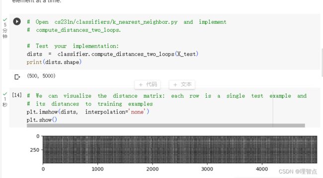
Inline Question 1
题面

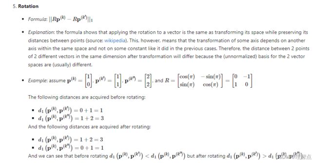
请注意距离矩阵中的结构化图案,其中一些行或列明显更亮。(请注意,在默认配色方案中,黑色表示低距离,而白色表示高距离。)
解答
-
是什么导致了一行中的数据明亮
从图像中我们可以看到这个图像是500 * 5000的一个图像,对于第 i 行而言,就等于第 i 个测试图像,与所有训练图像的L2距离,而明亮就说明他的L2距离比较大,也就是偏差比较大
-
是什么导致了一列中的数据明亮
同上,只不是这次是对于第 j 个训练数据而言,与500个测试数据的L2距离比较大
predict_labels
题面

解析
让我们用上一个函数求得的dist来算出对于每一个测试数据而言,L2距离最小的训练数据对应的标签
并且题目中已经给了我们提示,让我们使用numpy.argsort来实现
- numpy.argsort() 函数用于使用关键字kind指定的算法沿给定轴执行间接排序。 它返回一个与 arr 形状相同的索引数组,用于对数组进行排序,按升序排列
- 函数原型
numpy.argsort(arr, axis=-1, kind=’quicksort’, order=None)
- 参数
- arr:[array_like],输入数组
- axis:[int or None],排序的轴, 如果没有,数组在排序前被展平。 默认值为 -1,即沿最后一个轴排序。
- kind:[‘quicksort’, ‘mergesort’, ‘heapsort’],选择算法, 默认为“快速排序”。
- order : [str or list of str] ,当 arr 是一个定义了字段的数组时,这个参数指定首先比较哪些字段,第二个等等。
- return: [index_array, ndarray] ,沿指定轴对 arr 排序的索引数组。如果 arr 是一维的,则 arr[index_array] 返回排序后的 arr。
实例代码
# get two largest value from numpy array
x=np.array([12,43,2,100,54,5,68])
print(x)
# using argsort get indices of value of arranged in ascending order
print(np.argsort(x))
#get two highest value index of array
print(np.argsort(x)[-2:])
# to arrange in ascending order of index
print(np.argsort(x)[-2:][::-1])
# to get highest 2 values from array
x[np.argsort(x)[-2:][::-1]]
输出
[ 12  43   2 100  54   5  68]
[2 5 0 1 4 6 3]
[6 3]
[3 6]
[100  68]
因此我们只要用一行代码就可以实现获取目标的下标
closest_y = self.y_train[np.argsort(dists[i])[:k]]
# np.argsort(dists[i])[:k] 就是最小的k个值的下标
# 这样子代码是已经获取到了最小的k个值对应的label了
之后让我们取出最为普遍的标签,也就是出现的最多的标签
接下来我们只需要使用np.bincount 和 np.argmax两个函数
np.bincount() 是一个用于计算整数数组中每个值出现次数的函数。它返回一个数组,其长度等于a中元素最大值加1,每个元素值则是它当前索引值在a中出现的次数。下面是一些示例代码和输出:
import numpy as np

a = np.array([0, 1, 2, 3, 2, 1, 5])
print(np.bincount(a)) # [1 2 2 1 0 1]

b = np.array([0,0,1,2,2])
print(np.bincount(b)) # [2 1 2]
np.argmax() 是一个用于返回数组中最大值的索引的函数。下面是一些示例代码和输出:
import numpy as np

a = np.array([1, 2, 3, 2, 1])
print(np.argmax(a)) # 2

b = np.array([5, 7, 3, 2], [8, 6, 4, 9])
print(np.argmax(b)) # 7
其实如果严谨的来说的话不应该用np.bincount的,因为如果k=3,但是我们选出来的前3个标签各不相同,那么应该选择最小的那个标签,但是使用Bincount的话无法保证这个情况,不过我懒得写复杂的方法了,而且对于分类算法而言,这点误差可以忽略不计,因为出现上面这种情况的话,就是分类效果不好 ^_^
代码
def predict_labels(self, dists, k=1):
        """
        Given a matrix of distances between test points and training points,
        predict a label for each test point.

        Inputs:
        - dists: A numpy array of shape (num_test, num_train) where dists[i, j]
          gives the distance betwen the ith test point and the jth training point.

        Returns:
        - y: A numpy array of shape (num_test,) containing predicted labels for the
          test data, where y[i] is the predicted label for the test point X[i].
        """
        num_test = dists.shape[0]
        y_pred = np.zeros(num_test)
        for i in range(num_test):
            # A list of length k storing the labels of the k nearest neighbors to
            # the ith test point.
            closest_y = []
            #########################################################################
            # TODO:                                                                 #
            # Use the distance matrix to find the k nearest neighbors of the ith    #
            # testing point, and use self.y_train to find the labels of these       #
            # neighbors. Store these labels in closest_y.                           #
            # Hint: Look up the function numpy.argsort.                             #
            #########################################################################
            # *****START OF YOUR CODE (DO NOT DELETE/MODIFY THIS LINE)*****

            closest_y = self.y_train[np.argsort(dists[i])[:k]]


            # *****END OF YOUR CODE (DO NOT DELETE/MODIFY THIS LINE)*****
            #########################################################################
            # TODO:                                                                 #
            # Now that you have found the labels of the k nearest neighbors, you    #
            # need to find the most common label in the list closest_y of labels.   #
            # Store this label in y_pred[i]. Break ties by choosing the smaller     #
            # label.                                                                #
            #########################################################################
            # *****START OF YOUR CODE (DO NOT DELETE/MODIFY THIS LINE)*****

            y_pred[i] = np.argmax(np.bincount(closest_y))

            # *****END OF YOUR CODE (DO NOT DELETE/MODIFY THIS LINE)*****

        return y_pred
结果
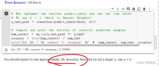
跟要求的也差不多,27%
Inline Question 2
题面

就是说
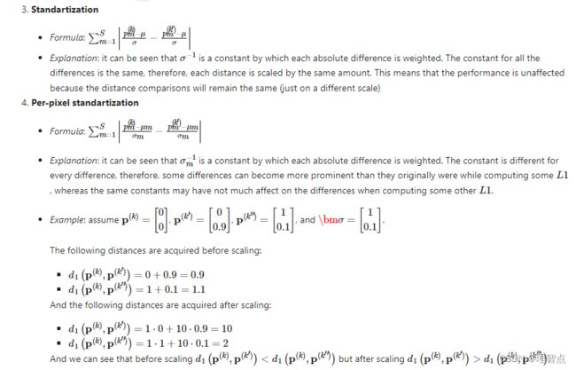
以下哪一个预处理步骤不会改变使用L1距离的最近邻分类器的性能?选择所有适用的选项。为了澄清,训练和测试示例都以相同的方式进行了预处理。
- 减去平均值μ(p~(k)ij=p(k)ij-μ。)
- 减去每像素平均值μij(p~(k)ij=p(k)ij-μij.)
- 减去平均值μ,除以标准偏差σ。
- 减去像素平均值μij,除以像素标准偏差σij。
- 旋转数据的坐标轴,这意味着将所有图像旋转相同的角度。图像中由旋转引起的空区域用相同的像素值填充,并且不执行插值。
解答
这个问题恕鄙人不才,因为我也不是特别理解这段,我一开始觉得答案是1、2、3、4,但是网上的答案五花八门(可恶啊不是斯坦福的学生不能享受人家的解答),后来我找到一个比较官方的解答,我直接把他的回答粘贴过来了(英文的,我就不翻译了,怕产生歧义)

compute_distances_one_loop
题面

解答
就是让我们只用一个循环来实现计算L2距离,没啥好说的,还是考察的np的用法
代码
    def compute_distances_one_loop(self, X):
        """
        Compute the distance between each test point in X and each training point
        in self.X_train using a single loop over the test data.

        Input / Output: Same as compute_distances_two_loops
        """
        num_test = X.shape[0]
        num_train = self.X_train.shape[0]
        dists = np.zeros((num_test, num_train))
        for i in range(num_test):
            #######################################################################
            # TODO:                                                               #
            # Compute the l2 distance between the ith test point and all training #
            # points, and store the result in dists[i, :].                        #
            # Do not use np.linalg.norm().                                        #
            #######################################################################
            # *****START OF YOUR CODE (DO NOT DELETE/MODIFY THIS LINE)*****

            dists[i,:] = np.sqrt(np.sum(np.power(self.X_train - X[i],2),axis=1))

            # *****END OF YOUR CODE (DO NOT DELETE/MODIFY THIS LINE)*****
        return dists
compute_distances_no_loops
题面

让我们不使用循环来实现求解
解析
自己稍加思考加上我上面的解析应该能懂,如果又不懂的地方可以联系我
代码
def compute_distances_no_loops(self, X):
        """
        Compute the distance between each test point in X and each training point
        in self.X_train using no explicit loops.

        Input / Output: Same as compute_distances_two_loops
        """
        num_test = X.shape[0]
        num_train = self.X_train.shape[0]
        dists = np.zeros((num_test, num_train))
        #########################################################################
        # TODO:                                                                 #
        # Compute the l2 distance between all test points and all training      #
        # points without using any explicit loops, and store the result in      #
        # dists.                                                                #
        #                                                                       #
        # You should implement this function using only basic array operations; #
        # in particular you should not use functions from scipy,                #
        # nor use np.linalg.norm().                                             #
        #                                                                       #
        # HINT: Try to formulate the l2 distance using matrix multiplication    #
        #       and two broadcast sums.                                         #
        #########################################################################
        # *****START OF YOUR CODE (DO NOT DELETE/MODIFY THIS LINE)*****

        tmp1 = np.sum(np.power(X,2),axis=1).reshape((X.shape[0],1))
        tmp2 = np.sum(np.power(self.X_train,2),axis = 1).reshape((self.X_train.shape[0],1)).T
        dists = np.sqrt(-2 * (X @ self.X_train.T) + tmp1 + tmp2)
        # print(dists.shape)
        # print(tmp1.shape)
        # print(tmp2.shape)

        # *****END OF YOUR CODE (DO NOT DELETE/MODIFY THIS LINE)*****
        return dists
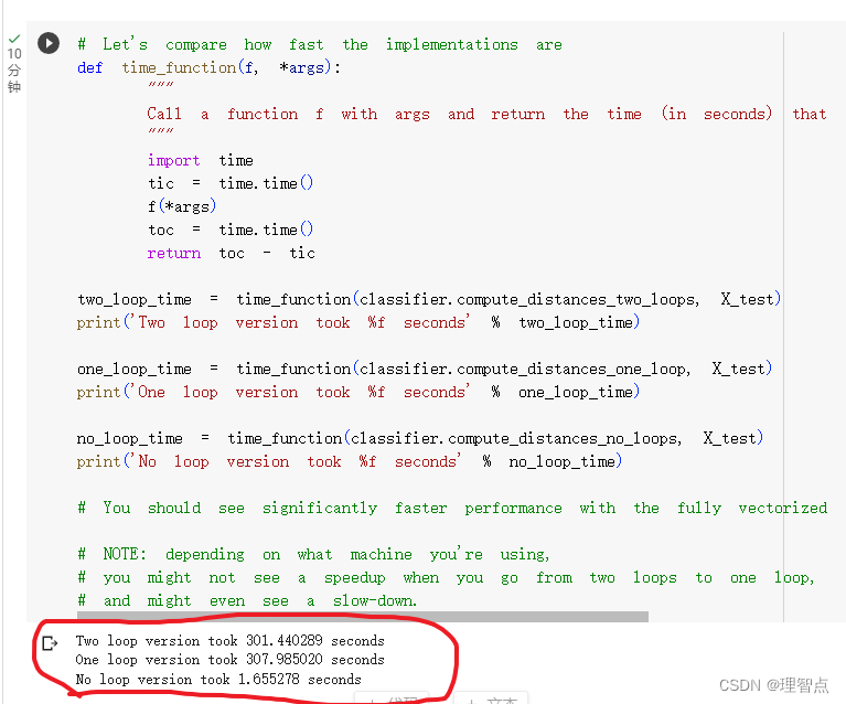
最后可以看到时间确实快了很多
Cross-validation
题面
就是让我们实现视频里一样的交叉校验
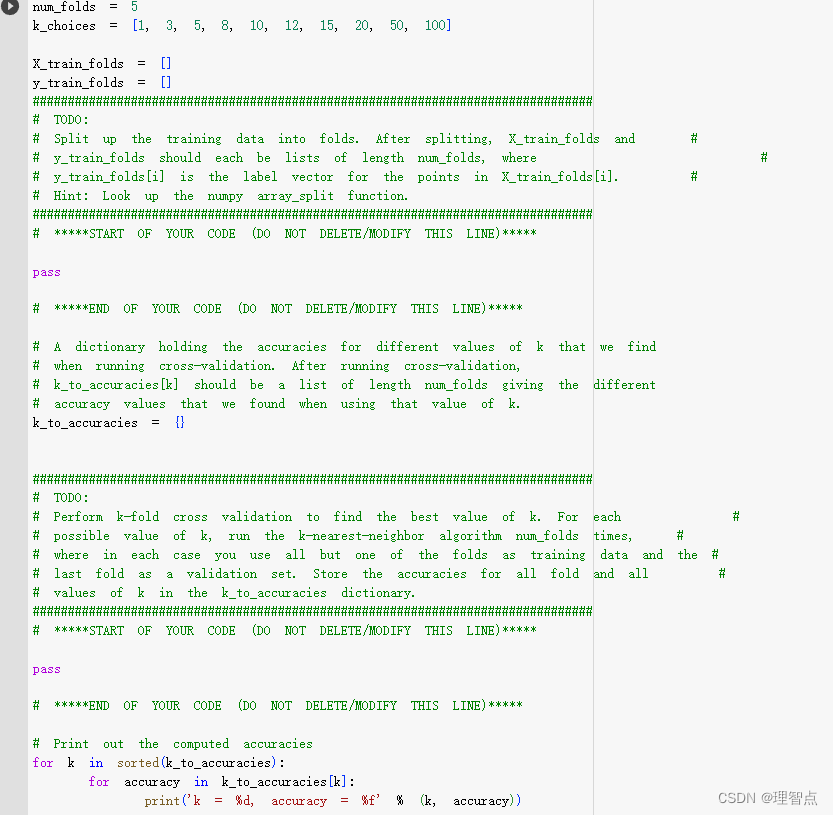
任务一
将训练数据切分成不同的折。切分之后,训练样本和对应的样本标签被包含在数组 X_train_folds和y_train_folds之中,数组长度是折数num_folds。其中 y_train_folds[i]是一个矢量,表示矢量X_train_folds[i]中所有样本的标签
提示: 可以尝试使用numpy的array_split方法。
任务二:
通过k折的交叉验证找到最佳k值。对于每一个k值,执行kNN算法num_folds次,每一次执行中,选择一折为验证集,其它折为训练集。将不同k值在不同折上的验证结果保存在k_to_accuracies字典中。
代码
num_folds = 5
k_choices = [1, 3, 5, 8, 10, 12, 15, 20, 50, 100]

X_train_folds = []
y_train_folds = []
################################################################################
# TODO:                                                                        #
# Split up the training data into folds. After splitting, X_train_folds and    #
# y_train_folds should each be lists of length num_folds, where                #
# y_train_folds[i] is the label vector for the points in X_train_folds[i].     #
# Hint: Look up the numpy array_split function.                                #
################################################################################
# *****START OF YOUR CODE (DO NOT DELETE/MODIFY THIS LINE)*****

X_train_folds = np.array_split(X_train,num_folds)
y_train_folds = np.array_split(y_train,num_folds)
# print(X_train_folds)

# *****END OF YOUR CODE (DO NOT DELETE/MODIFY THIS LINE)*****

# A dictionary holding the accuracies for different values of k that we find
# when running cross-validation. After running cross-validation,
# k_to_accuracies[k] should be a list of length num_folds giving the different
# accuracy values that we found when using that value of k.
k_to_accuracies = {}


################################################################################
# TODO:                                                                        #
# Perform k-fold cross validation to find the best value of k. For each        #
# possible value of k, run the k-nearest-neighbor algorithm num_folds times,   #
# where in each case you use all but one of the folds as training data and the #
# last fold as a validation set. Store the accuracies for all fold and all     #
# values of k in the k_to_accuracies dictionary.                               #
################################################################################
# *****START OF YOUR CODE (DO NOT DELETE/MODIFY THIS LINE)*****

pass
for k in k_choices:
  k_to_accuracies[k] = []
  for i in range(num_folds):
    #选择第i个分片为验证集,其他数据为训练数据
    temp_train_x = np.concatenate(np.compress([False if temp_i == i else True for temp_i in range(num_folds)],X_train_folds,axis=0))
    temp_train_y = np.concatenate(np.compress([False if temp_i == i else True for temp_i in range(num_folds)],y_train_folds,axis=0))

    # 训练数据
    classifier.train(temp_train_x,temp_train_y)

    # 获取预测
    temp_pred_y = classifier.predict(X_train_folds[i],k=k,num_loops=0)

    # 计算准确率
    correct_count = np.sum(temp_pred_y == y_train_folds[i])
    k_to_accuracies[k].append(correct_count / len(temp_pred_y))


# *****END OF YOUR CODE (DO NOT DELETE/MODIFY THIS LINE)*****

# Print out the computed accuracies
for k in sorted(k_to_accuracies):
    for accuracy in k_to_accuracies[k]:
        print('k = %d, accuracy = %f' % (k, accuracy))
解析
没啥好说的,就是按照题目意思完成就好了
输出

最后
最后还有一题解答题懒得做的,这个题目做的没啥意思。
Q2 Training a Support Vector Machine
就是让我们学习并使用svm算法
svm算法如下图所示
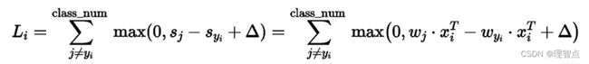
其中
Wj * Xi 是错误分类的分数
-Wyi * Xi 是正确分类的分数
所以一旦分类错误,就可以计算出对于该损失函数的梯度
其中正确分类的Wj所在的梯度是 -Xi
错误分类的Wyi所在的梯度是 +Xi
svm_loss_naive
题面
解析
就是让我们计算梯度,具体的梯度是多少,我已经在上面写出来了
代码
def svm_loss_naive(W, X, y, reg):
"""
Structured SVM loss function, naive implementation (with loops).
Inputs have dimension D, there are C classes, and we operate on minibatches
of N examples.
Inputs:
- W: A numpy array of shape (D, C) containing weights.
- X: A numpy array of shape (N, D) containing a minibatch of data.
- y: A numpy array of shape (N,) containing training labels; y[i] = c means
that X[i] has label c, where 0 <= c < C.
- reg: (float) regularization strength
Returns a tuple of:
- loss as single float
- gradient with respect to weights W; an array of same shape as W
"""
dW = np.zeros(W.shape) # initialize the gradient as zero
# compute the loss and the gradient
num_classes = W.shape[1]
num_train = X.shape[0]
loss = 0.0
for i in range(num_train):
scores = X[i].dot(W)
correct_class_score = scores[y[i]]
for j in range(num_classes):
if j == y[i]:
continue
margin = scores[j] - correct_class_score + 1 # note delta = 1
if margin > 0:
loss += margin
# 正确分类的梯度减上X[i]
dW[:,y[i]] -= X[i].T
# 错误分类的梯度加去X[i]
dW[:,j] += X[i].T
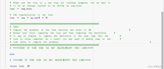
# Right now the loss is a sum over all training examples, but we want it
# to be an average instead so we divide by num_train.
loss /= num_train
# Add regularization to the loss.
loss += reg * np.sum(W * W)
#############################################################################
# TODO: #
# Compute the gradient of the loss function and store it dW. #
# Rather that first computing the loss and then computing the derivative, #
# it may be simpler to compute the derivative at the same time that the #
# loss is being computed. As a result you may need to modify some of the #
# code above to compute the gradient. #
#############################################################################
# *****START OF YOUR CODE (DO NOT DELETE/MODIFY THIS LINE)*****
# 梯度同样处理
dW /= num_train
# 正则项的梯度
dW += 2 * reg * W
# *****END OF YOUR CODE (DO NOT DELETE/MODIFY THIS LINE)*****
return loss, dW
svm_loss_vectorized (loss)
题面
就是让我们用向量法来计算loss而不是用循环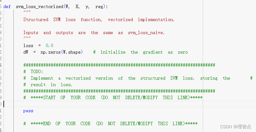
解析
解析写到代码注释里了,稍微思考下就能理解了
代码
def svm_loss_vectorized(W, X, y, reg):
"""
Structured SVM loss function, vectorized implementation.
Inputs and outputs are the same as svm_loss_naive.
"""
loss = 0.0
dW = np.zeros(W.shape) # initialize the gradient as zero
#############################################################################
# TODO: #
# Implement a vectorized version of the structured SVM loss, storing the #
# result in loss. #
#############################################################################
# *****START OF YOUR CODE (DO NOT DELETE/MODIFY THIS LINE)*****
num_classes = W.shape[1]
num_train = X.shape[0]
scores = X @ W
# 获取对于每个x而言正确分类的分数
scores_correct = scores[range(num_train),y].reshape((scores.shape[0],1))
# 对每个元素做max(0,scores_error - scores_correct + 1)操作,包括正确分类的元素
# 统一操作后减少代码编写难度,只需要最后处理一下正确分类的分数,把他们变成0就行了
margins = np.maximum(0,scores - scores_correct + 1)
# 将正确分类的margins置为0
margins[range(num_train),y] = 0
loss += np.sum(margins) / num_train
loss += reg * np.sum(W * W)
# *****END OF YOUR CODE (DO NOT DELETE/MODIFY THIS LINE)*****
#############################################################################
# TODO: #
# Implement a vectorized version of the gradient for the structured SVM #
# loss, storing the result in dW. #
# #
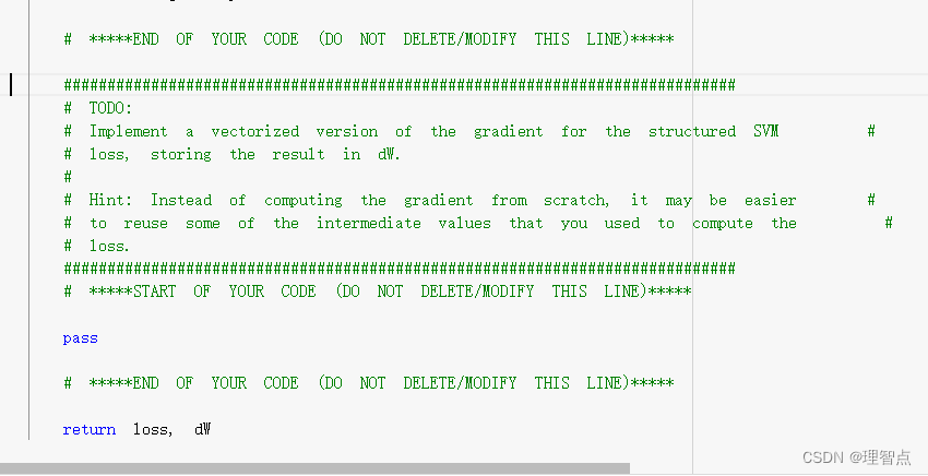
# Hint: Instead of computing the gradient from scratch, it may be easier #
# to reuse some of the intermediate values that you used to compute the #
# loss. #
#############################################################################
# *****START OF YOUR CODE (DO NOT DELETE/MODIFY THIS LINE)*****
pass
# *****END OF YOUR CODE (DO NOT DELETE/MODIFY THIS LINE)*****
return loss, dW
输出

svm_loss_vectorized (gradient)
题面
解析
解析写到代码注释里了,这个问题还是需要一点思考的,如果觉得我的注释看不懂可以联系我,我画图解释一下,但是建议还是自己思考
代码
def svm_loss_vectorized(W, X, y, reg):
    """
    Structured SVM loss function, vectorized implementation.

    Inputs and outputs are the same as svm_loss_naive.
    """
    loss = 0.0
    dW = np.zeros(W.shape)  # initialize the gradient as zero

    #############################################################################
    # TODO:                                                                     #
    # Implement a vectorized version of the structured SVM loss, storing the    #
    # result in loss.                                                           #
    #############################################################################
    # *****START OF YOUR CODE (DO NOT DELETE/MODIFY THIS LINE)*****

    num_classes = W.shape[1]
    num_train = X.shape[0]

    scores = X @ W
    # 获取对于每个x而言正确分类的分数
    scores_correct = scores[range(num_train),y].reshape((scores.shape[0],1))
    # 对每个元素做max(0,scores_error - scores_correct + 1)操作,包括正确分类的元素
    # 统一操作后减少代码编写难度,只需要最后处理一下正确分类的分数,把他们变成0就行了
    margins = np.maximum(0,scores - scores_correct + 1)
    # 将正确分类的margins置为0
    margins[range(num_train),y] = 0
    loss += np.sum(margins) / num_train
    loss += reg * np.sum(W * W)

    # *****END OF YOUR CODE (DO NOT DELETE/MODIFY THIS LINE)*****

    #############################################################################
    # TODO:                                                                     #
    # Implement a vectorized version of the gradient for the structured SVM     #
    # loss, storing the result in dW.                                           #
    #                                                                           #
    # Hint: Instead of computing the gradient from scratch, it may be easier    #
    # to reuse some of the intermediate values that you used to compute the     #
    # loss.                                                                     #
    #############################################################################
    # *****START OF YOUR CODE (DO NOT DELETE/MODIFY THIS LINE)*****

    # 先把所有margins > 0 的标记为1 ,因为我们算梯度的时候并不需要用到具体的元素的loss是多少
    # 我们只想知道这个元素有没有被算进loss里面
    margins[margins > 0] = 1
    # 并且,对于每一个分类错误的元素而言,他对错误分类的W的梯度影响是 +X[i]
    # 他对正确分类的W的梯度影响是-X[i]
    # 并且正确分类的分数位置我们是知道的
    # 因此我们只需要计算对于X[i]而言,有多少个分类 > 0,就代表错误分类的个数
    # 这个数量就是影响了梯度的数量,并且我们已经把错误分类的位置记为了1
    # 接下来我们只要做到在正确分类的位置 - 错误分类的个数
    # 接下来是举例,一直我们一共有10个分类,对于X[i]而言,我们有3个分类正确,加上一个本来就是正确分类的分数
    # 那么剩下6个分类错误的,也就是错误分类的预估值> 正确分类的预估值 - 1 的数量
    # 那么对于梯度而言,我们只需要对正确分类的梯度 减去六个X[i]就行,错误分类的个数各自 加上一个X[i],具体的结合矩阵的shape
    # 思考一下,如果实在理解不了可以给我留言,我画个图
    row_sum = np.sum(margins,axis = 1)
    margins[range(num_train),y] = -row_sum
    dW += np.dot(X.T, margins)/num_train + reg * W


    # *****END OF YOUR CODE (DO NOT DELETE/MODIFY THIS LINE)*****

    return loss, dW
输出

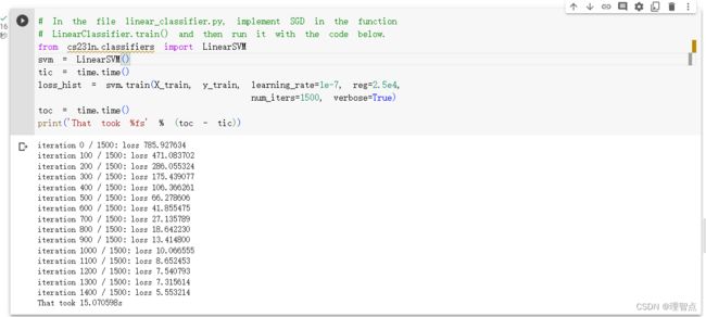
LinearClassifier.train
题面
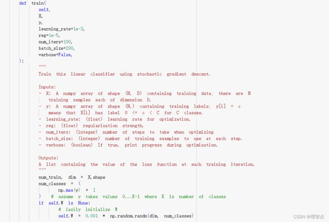
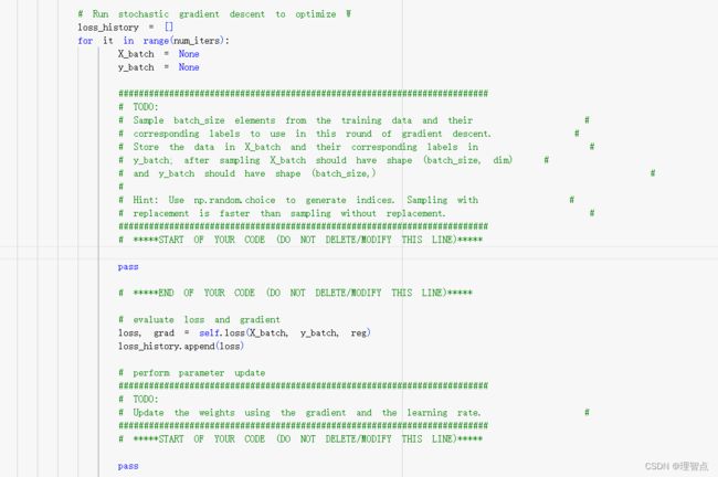

就是让我们实现两件事,一个是随机采样训练数据,另一个就是实现权值的更新
解析
这个没啥好说的,正常写就完了,没有难的点,有不会的地方再去看视频学习
代码
def train(
        self,
        X,
        y,
        learning_rate=1e-3,
        reg=1e-5,
        num_iters=100,
        batch_size=200,
        verbose=False,
    ):
        """
        Train this linear classifier using stochastic gradient descent.

        Inputs:
        - X: A numpy array of shape (N, D) containing training data; there are N
          training samples each of dimension D.
        - y: A numpy array of shape (N,) containing training labels; y[i] = c
          means that X[i] has label 0 <= c < C for C classes.
        - learning_rate: (float) learning rate for optimization.
        - reg: (float) regularization strength.
        - num_iters: (integer) number of steps to take when optimizing
        - batch_size: (integer) number of training examples to use at each step.
        - verbose: (boolean) If true, print progress during optimization.

        Outputs:
        A list containing the value of the loss function at each training iteration.
        """
        num_train, dim = X.shape
        num_classes = (
            np.max(y) + 1
        )  # assume y takes values 0...K-1 where K is number of classes
        if self.W is None:
            # lazily initialize W
            self.W = 0.001 * np.random.randn(dim, num_classes)

        # Run stochastic gradient descent to optimize W
        loss_history = []
        for it in range(num_iters):
            X_batch = None
            y_batch = None

            #########################################################################
            # TODO:                                                                 #
            # Sample batch_size elements from the training data and their           #
            # corresponding labels to use in this round of gradient descent.        #
            # Store the data in X_batch and their corresponding labels in           #
            # y_batch; after sampling X_batch should have shape (batch_size, dim)   #
            # and y_batch should have shape (batch_size,)                           #
            #                                                                       #
            # Hint: Use np.random.choice to generate indices. Sampling with         #
            # replacement is faster than sampling without replacement.              #
            #########################################################################
            # *****START OF YOUR CODE (DO NOT DELETE/MODIFY THIS LINE)*****

            choice_idxs = np.random.choice(num_train,batch_size)
            X_batch = X[choice_idxs]
            y_batch = y[choice_idxs]

            # *****END OF YOUR CODE (DO NOT DELETE/MODIFY THIS LINE)*****

            # evaluate loss and gradient
            loss, grad = self.loss(X_batch, y_batch, reg)
            loss_history.append(loss)

            # perform parameter update
            #########################################################################
            # TODO:                                                                 #
            # Update the weights using the gradient and the learning rate.          #
            #########################################################################
            # *****START OF YOUR CODE (DO NOT DELETE/MODIFY THIS LINE)*****

            self.W -= learning_rate * grad

            # *****END OF YOUR CODE (DO NOT DELETE/MODIFY THIS LINE)*****

            if verbose and it % 100 == 0:
                print("iteration %d / %d: loss %f" % (it, num_iters, loss))

        return loss_history
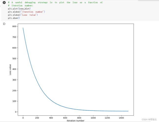
输出
predict
题面
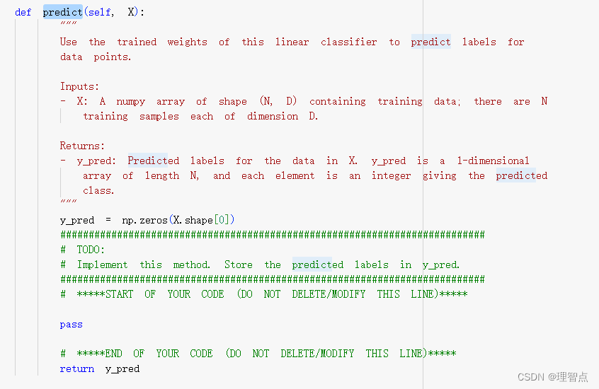
就是一个很简单的让我们使用之前实现的svm来进行预测
代码
def predict(self, X):
        """
        Use the trained weights of this linear classifier to predict labels for
        data points.

        Inputs:
        - X: A numpy array of shape (N, D) containing training data; there are N
          training samples each of dimension D.

        Returns:
        - y_pred: Predicted labels for the data in X. y_pred is a 1-dimensional
          array of length N, and each element is an integer giving the predicted
          class.
        """
        y_pred = np.zeros(X.shape[0])
        ###########################################################################
        # TODO:                                                                   #
        # Implement this method. Store the predicted labels in y_pred.            #
        ###########################################################################
        # *****START OF YOUR CODE (DO NOT DELETE/MODIFY THIS LINE)*****

        scores = X @ self.W
        y_pred = np.argmax(scores,axis= 1)

        # *****END OF YOUR CODE (DO NOT DELETE/MODIFY THIS LINE)*****
        return y_pred
输出
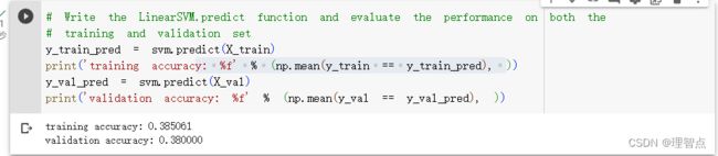
找到最好的hypeparameter
题面

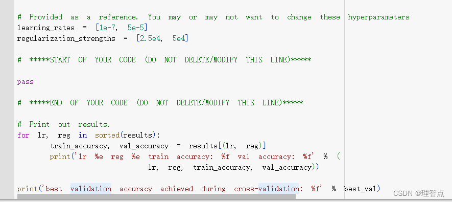
就是让我们自己试出最好的learning_rate 和 reg ,然后将结果保存到result中
代码
# Use the validation set to tune hyperparameters (regularization strength and
# learning rate). You should experiment with different ranges for the learning
# rates and regularization strengths; if you are careful you should be able to
# get a classification accuracy of about 0.39 (> 0.385) on the validation set.
# Note: you may see runtime/overflow warnings during hyper-parameter search.
# This may be caused by extreme values, and is not a bug.
# results is dictionary mapping tuples of the form
# (learning_rate, regularization_strength) to tuples of the form
# (training_accuracy, validation_accuracy). The accuracy is simply the fraction
# of data points that are correctly classified.
results = {}
best_val = -1 # The highest validation accuracy that we have seen so far.
best_svm = None # The LinearSVM object that achieved the highest validation rate.
################################################################################
# TODO: #
# Write code that chooses the best hyperparameters by tuning on the validation #
# set. For each combination of hyperparameters, train a linear SVM on the #
# training set, compute its accuracy on the training and validation sets, and #
# store these numbers in the results dictionary. In addition, store the best #
# validation accuracy in best_val and the LinearSVM object that achieves this #
# accuracy in best_svm. #
# #
# Hint: You should use a small value for num_iters as you develop your #
# validation code so that the SVMs don't take much time to train; once you are #
# confident that your validation code works, you should rerun the validation #
# code with a larger value for num_iters. #
################################################################################
# Provided as a reference. You may or may not want to change these hyperparameters
learning_rates = [2e-7, 0.75e-7,1.5e-7, 1.25e-7, 0.75e-7]
regularization_strengths = [3e4, 3.25e4, 3.5e4, 3.75e4, 4e4,4.25e4, 4.5e4,4.75e4, 5e4]
# *****START OF YOUR CODE (DO NOT DELETE/MODIFY THIS LINE)*****
for lr in learning_rates:
for reg in regularization_strengths:
svm = LinearSVM()
svm.train(X_train, y_train, learning_rate=lr, reg=reg,num_iters=1500, verbose=False)
y_train_pred = svm.predict(X_train)
y_train_accuracy = np.mean(y_train == y_train_pred)
y_val_pred = svm.predict(X_val)
y_val_accuracy = np.mean(y_val == y_val_pred)
results[(lr,reg)] = (y_train_accuracy,y_val_accuracy)
if(y_val_accuracy > best_val):
best_val = y_val_accuracy
best_svm = svm
# *****END OF YOUR CODE (DO NOT DELETE/MODIFY THIS LINE)*****
# Print out results.
for lr, reg in sorted(results):
train_accuracy, val_accuracy = results[(lr, reg)]
print('lr %e reg %e train accuracy: %f val accuracy: %f' % (
lr, reg, train_accuracy, val_accuracy))
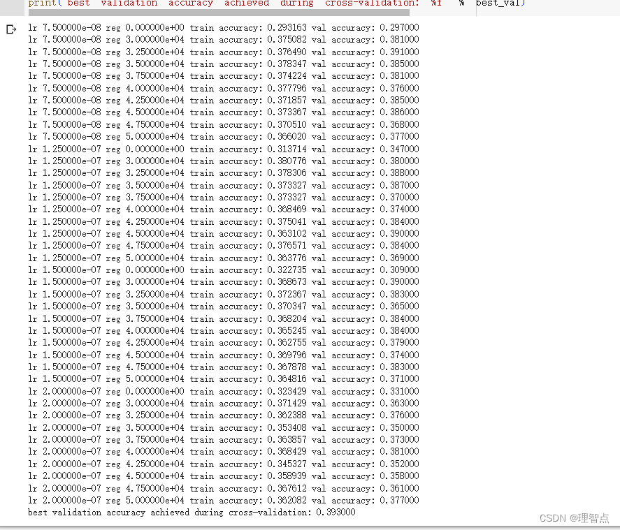
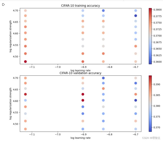
print('best validation accuracy achieved during cross-validation: %f' % best_val)
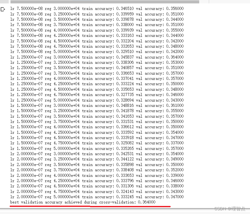
输出
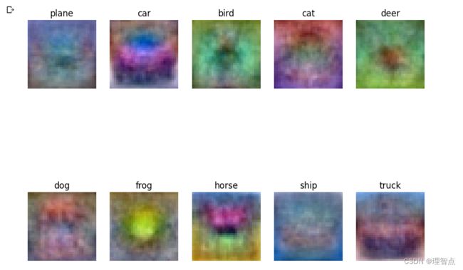
最后输出最后的结果

Q3 softmax
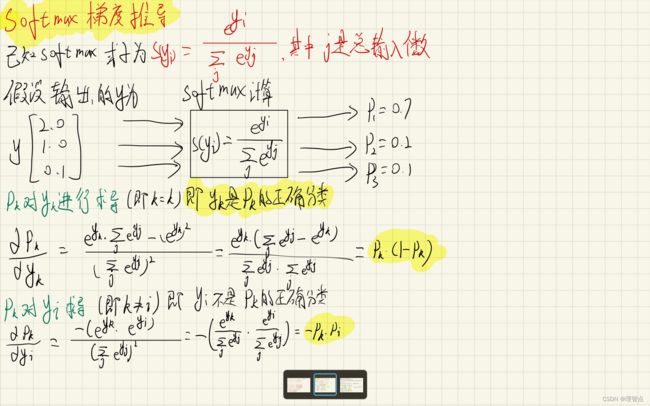
softmax 讲解与梯度推导

softmax_loss_naive
题面
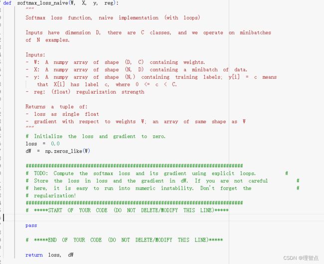
让我们用简单写法来实现softmax的loss函数与梯度计算
解析
写到代码注释里了,结合上面的讲解来看,还看不懂就看课
代码
def softmax_loss_naive(W, X, y, reg):
    """
    Softmax loss function, naive implementation (with loops)

    Inputs have dimension D, there are C classes, and we operate on minibatches
    of N examples.

    Inputs:
    - W: A numpy array of shape (D, C) containing weights.
    - X: A numpy array of shape (N, D) containing a minibatch of data.
    - y: A numpy array of shape (N,) containing training labels; y[i] = c means
      that X[i] has label c, where 0 <= c < C.
    - reg: (float) regularization strength

    Returns a tuple of:
    - loss as single float
    - gradient with respect to weights W; an array of same shape as W
    """
    # Initialize the loss and gradient to zero.
    loss = 0.0
    dW = np.zeros_like(W)

    #############################################################################
    # TODO: Compute the softmax loss and its gradient using explicit loops.     #
    # Store the loss in loss and the gradient in dW. If you are not careful     #
    # here, it is easy to run into numeric instability. Don't forget the        #
    # regularization!                                                           #
    #############################################################################
    # *****START OF YOUR CODE (DO NOT DELETE/MODIFY THIS LINE)*****

    # 训练集的数量
    num_train = X.shape[0]
    # 分类的数量
    num_classes = W.shape[1]
    for i in range(num_train):
      scores = X[i] @ W
      # 对其求e的幂函数
      scores = np.exp(scores)
      # 求对于每一个分类的概率
      p = scores / np.sum(scores)
      # 求loss函数
      loss += -np.log(p[y[i]])

      # 求梯度
      for k in range(num_classes):
        # 获取当前分类的概率
        p_k = p[k]
        # 判断当前分类是否是正确分类
        if k == y[i]:
          dW[:,k] += (p_k - 1) * X[i]
        else:
          dW[:,k] += (p_k) * X[i]


    # 处理正则项
    loss /= num_train
    dW /= num_train
    loss += 0.5 * reg * np.sum(W * W)
    dW += reg * W


    # *****END OF YOUR CODE (DO NOT DELETE/MODIFY THIS LINE)*****

    return loss, dW
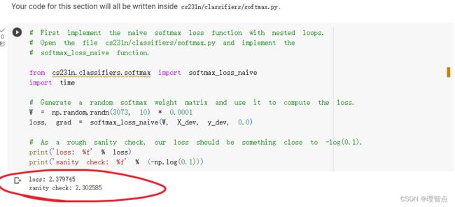
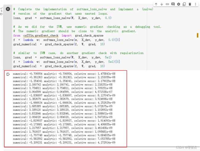
结果
softmax_loss_vectorized
题面
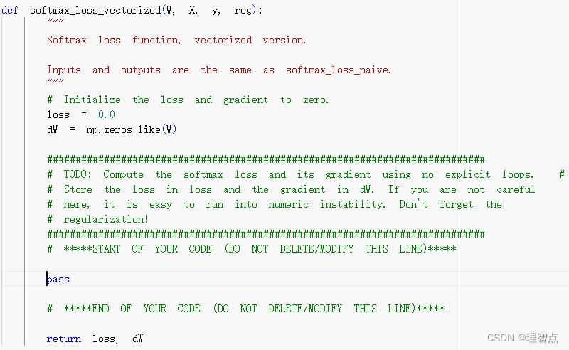
就是让我们使用序列化的方式来实现softmax
解析
解析写代码注释里了,注意这部分的梯度计算课上没讲,你得自己手推一遍才能理解,具体的可以看上面的softmax 讲解与梯度推导
代码
def softmax_loss_vectorized(W, X, y, reg):
    """
    Softmax loss function, vectorized version.

    Inputs and outputs are the same as softmax_loss_naive.
    """
    # Initialize the loss and gradient to zero.
    loss = 0.0
    dW = np.zeros_like(W)

    #############################################################################
    # TODO: Compute the softmax loss and its gradient using no explicit loops.  #
    # Store the loss in loss and the gradient in dW. If you are not careful     #
    # here, it is easy to run into numeric instability. Don't forget the        #
    # regularization!                                                           #
    #############################################################################
    # *****START OF YOUR CODE (DO NOT DELETE/MODIFY THIS LINE)*****

    # 训练集的数量
    num_train = X.shape[0]
    # 分类的数量
    num_classes = W.shape[1]

    # 先计算得分
    scores = X @ W
    # 再取e的幂函数
    scores = np.exp(scores)
    # 计算所有的概率
    p = scores / np.sum(scores,axis = 1,keepdims = True)
    # 计算loss函数
    loss += np.sum(-np.log(p[range(num_train),y]))

    # 计算梯度 根据上面的公式可以知道只要给正确分类的P - 1就可以得到dW
    p[range(num_train),y] -= 1
    dW = X.T @ p


    # 计算正则项
    loss /= num_train
    loss += 0.5 * reg * np.sum(W * W)

    dW /= num_train
    dW += reg * W
    # *****END OF YOUR CODE (DO NOT DELETE/MODIFY THIS LINE)*****

    return loss, dW
找到最好的hypeparameter
题面

解析
跟q2的一样
代码
# Use the validation set to tune hyperparameters (regularization strength and
# learning rate). You should experiment with different ranges for the learning
# rates and regularization strengths; if you are careful you should be able to
# get a classification accuracy of over 0.35 on the validation set.

from cs231n.classifiers import Softmax
results = {}
best_val = -1
best_softmax = None

################################################################################
# TODO:                                                                        #
# Use the validation set to set the learning rate and regularization strength. #
# This should be identical to the validation that you did for the SVM; save    #
# the best trained softmax classifer in best_softmax.                          #
################################################################################

# Provided as a reference. You may or may not want to change these hyperparameters
learning_rates = [2e-7, 0.75e-7,1.5e-7, 1.25e-7, 0.75e-7]
regularization_strengths = [3e4, 3.25e4, 3.5e4, 3.75e4, 4e4,4.25e4, 4.5e4,4.75e4, 5e4]

# *****START OF YOUR CODE (DO NOT DELETE/MODIFY THIS LINE)*****

for lr in learning_rates:
  for reg in regularization_strengths:
    softmax = Softmax()
    softmax.train(X_train, y_train, learning_rate=lr, reg=reg,num_iters=1500, verbose=False)
    y_train_pred = softmax.predict(X_train)
    y_train_accuracy = np.mean(y_train == y_train_pred)
    y_val_pred = softmax.predict(X_val)
    y_val_accuracy = np.mean(y_val == y_val_pred)
    results[(lr,reg)] = (y_train_accuracy,y_val_accuracy)
    if(y_val_accuracy > best_val):
      best_val = y_val_accuracy
      best_softmax = softmax

# *****END OF YOUR CODE (DO NOT DELETE/MODIFY THIS LINE)*****

# Print out results.
for lr, reg in sorted(results):
    train_accuracy, val_accuracy = results[(lr, reg)]
    print('lr %e reg %e train accuracy: %f val accuracy: %f' % (
                lr, reg, train_accuracy, val_accuracy))

print('best validation accuracy achieved during cross-validation: %f' % best_val)
输出
最后的结果