mpf11_Learning rate_Activation_Loss_Optimizer_Quadratic Program_NewtonTaylor_L-BFGS_Nesterov_Hessian
Deep learning represents the very cutting edge of Artificial Intelligence (AI). Unlike machine learning, deep learning takes a different approach in making predictions by using a neural network. An artificial neural network is modeled on the human nervous system, consisting of an input layer and an output layer, with one or more hidden layers in between. Each layer consists of artificial neurons working in parallel and passing outputs to the next layer as inputs. The word deep in deep learning comes from the notion that as data passes through more hidden layers in an artificial neural network, more complex features can be extracted.
TensorFlow is an open source, powerful machine learning and deep learning framework developed by Google. In this chapter, we will take a hands-on approach to learning TensorFlow by building a deep learning model with four hidden layers to predict the prices of a security. Deep learning models are trained by passing the entire dataset forward and backward through the network, with each iteration known as an epoch. Because the input data can be too big to be fed, training can be done in batches, and this process is known as mini-batch training.
Another popular deep learning library is Keras, which utilizes TensorFlow as the backend. We will also take a hands-on approach to learning Keras and see how easy it is to build a deep learning model to predict credit card payment defaults.
In this chapter, we will cover the following topics:
- An introduction to neural networks
- Neurons, activation functions, loss functions, and optimizers
- Different types of neural network architectures
- How to build security price prediction deep learning model using TensorFlow
- Keras, a user-friendly deep learning framework
- How to build credit card payment default prediction deep learning model using Keras
- How to display recorded events in a Keras history
A brief introduction to deep learning
The theory behind deep learning began as early as the 1940s. However, its popularity has soared/ sɔːrd /飙升 in recent years thanks in part to improvements in computing hardware technology, smarter algorithms, and the adoption of deep learning frameworks. There is much to cover beyond this book. This section serves as a quick guide to gain a working knowledge for following the examples that we will cover in later parts of this chapter.
What is deep learning ?
In https://blog.csdn.net/Linli522362242/article/details/126672904, Machine Learning for Finance, we learned how machine learning is useful for making predictions. Supervised learning uses error-minimization techniques to fit a model with training data, and can be regression based or classification based.
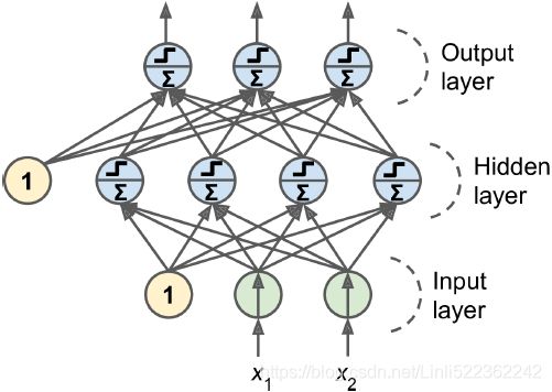
Deep learning takes a different approach in making predictions by using a neural network. Modeled on the human brain and the nervous system, an artificial neural network consists of a hierarchy of layers, with each layer made up of many simple units known as neurons, working in parallel and transforming the input data into abstract representations as the output data, which are fed to the next layer as input. The following diagram illustrates an artificial neural network:
Artificial neural networks consist of three types of layers. The first layer that accepts input is known as the input layer. The last layer where output is collected is known as the output layer. The layers between the input and output layers are known as hidden layers, since they are hidden from the interface of the network. There can be many combinations of hidden layers performing different activation functions. Naturally, more complex computations lead to a rise in demand for more powerful machines, such as the GPUs required to compute them.
The artificial neuron
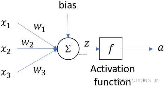
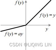
An artificial neuron receives one or more input and are multiplied by values known as weights, summed up and passed to an activation function. The final values computed by the activation function makes up the neuron's output. A bias value may be included in the summation term to help fit the data. The following diagram illustrates an artificial neuron:
 https://blog.csdn.net/Linli522362242/article/details/96480059
The summation term can be written as a linear equation such that ![]() . The neuron uses a nonlinear activation function
. The neuron uses a nonlinear activation function  to transform the input to become the output
  , and can be written as
 ![]() .
.
Activation function
(Linear,Sigmoid,Tanh,Hard tanh,ReLu,Leaky ReLU,PRelu,ELU,SELU,Softplus,Softsign)
An activation function is part of an artificial neuron that transforms the sum of weighted inputs into another value for the next layer. Usually, the range of this output value is -1 or 0 to 1. An artificial neuron is said to be activated when it passes a non-zero value to another neuron. There are several types of activation functions, mainly:
def sigmoid(z):
    return 1/(1+np.exp(-z))

def relu(z):
    return np.maximum( 0,z )

def softplus(z):
    return np.log( np.exp(z) +1.0 )

# Numerical Differentiation
# https://blog.csdn.net/Linli522362242/article/details/106290394
def derivative(f, z, eps=0.000001):
    # 1/2 * ( f(z+eps)-f(z)/eps + ( f(z)-f(z-eps) )/eps )
    # 1/2 * ( f(z+eps)/eps + f(z-eps)/eps )
    return ( f(z+eps) - f(z-eps) )/(2*eps)
import matplotlib.pyplot as plt
import numpy as np

z = np.linspace(-5, 5, 200)

plt.figure( figsize=(12,4) )

plt.subplot(121)
plt.plot( z, softplus(z), 'c:', linewidth=2, label='Softplus')
plt.plot( z, sigmoid(z), "y--", linewidth=2, label="Sigmoid" )
plt.plot( z, relu(z), "k-.", linewidth=2, label="ReLU" ) #ReLU (z) = max (0, z)
plt.plot( z, np.tanh(z), "b-", linewidth=2, label="Tanh" )
plt.plot( z, np.sign(z), "r-", linewidth=1, label="Step" )

plt.legend( loc="lower right", fontsize=14 )
plt.title("Activation function", fontsize=14 )
plt.axis([-5, 5, -1.5, 1.5])
# plt.axis('off')
plt.grid(visible=False)


plt.subplot(122)
plt.plot(0, 0, "ro", markersize=5)
#plt.plot(0, 0, "rx", markersize=10)

plt.plot( z, derivative(softplus, z), 'c:', linewidth=2, label='Softplus')
plt.plot(z, derivative(sigmoid, z), "y--", linewidth=2, label="sigmoid")
plt.plot(z, derivative( relu, z ), "k-.", linewidth=2, label="ReLU")
plt.plot(z, derivative(np.tanh, z), "b-", linewidth=2, label="Tanh")
plt.plot(z, derivative(np.sign, z), "r-", linewidth=1, label="Step")

plt.legend( loc="upper left", fontsize=14 )
plt.title("Derivatives", fontsize=14)
plt.axis([-5,5, -0.2, 1.5])
# plt.axis('off')
plt.grid(visible=False)


plt.show()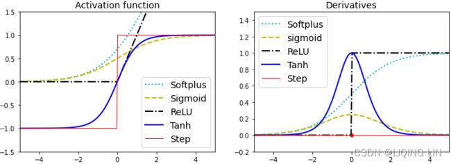
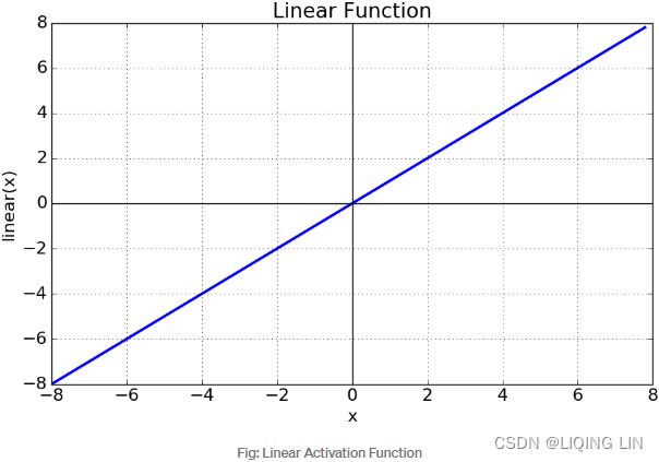
Linear : ###############
![]()
Sigmoid ( logistic sigmoid ) :
###############
https://towardsdatascience.com/derivative-of-the-sigmoid-function-536880cf918e![]() OR
OR![]()
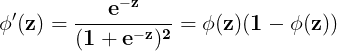 where
where ![]()
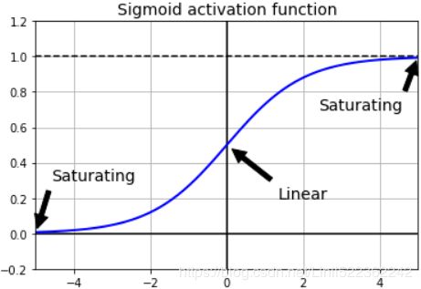
- 是一个平滑函数,并且具有连续性和可微性
- x轴在-3到3之间的梯度非常高,这意味着在[-3,3]这个范围内,x的少量变化也将导致y值的大幅度变化。因此,函数本质上试图将y值推向极值。 当我们尝试将值分类到特定的类时,使用Sigmoid函数非常理想。但是,一旦x值不在[-3,3]内,梯度就变得很小,接近于零,而网络就得不到真正的学习
- 优点:非线性;输出范围有限,适合作为输出层。 用于分类器时,Sigmoid函数及其组合通常效果更好
- 缺点:在两边太平滑,学习率太低;值总是正的;输出不是以0为中心(中心为0.5) 由于梯度消失问题,有时要避免使用sigmoid和tanh函数.
Tanh : ###############
![]()
![]()
The tanh functionis an alternative to the sigmoid function that is often found to converge faster in practice. The primary difference between tanh and sigmoid is that tanh output ranges from −1 to 1 while the sigmoid ranges from 0 to 1.
- has a mean of 0 and behaves slightly better than the logistic function
- 解决了sigmoid的大多数缺点(解决了所有值符号相同的问题),仍然有两边学习率太低的缺点. 其他属性都与sigmoid函数相同
Hard tanh : ###############
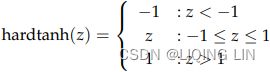

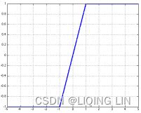
The hard tanh function is sometimes preferred over the tanh function since it is computationally cheaper. It does however saturate for magnitudes of z greater than 1. 
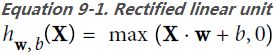
ReLu ( Rectified Linear Unit ): ###############

 OR
OR ![]()
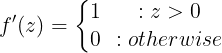
The ReLU (Rectified Linear Unit) function is a popular choice of activation since it does not saturate even for larger values of z and has found much success in computer vision applications:
- 首先,ReLU函数是非线性的,这意味着我们可以很容易地反向传播误差,并激活多个神经元
- 优点:不会同时激活所有的神经元,这意味着,在一段时间内,只有少量的神经元被激活 (如果输入值是负的,ReLU函数会转换为0,而神经元不被激活。),神经网络的这种稀疏性使其变得高效且易于计算. ReLU函数只能在隐藏层中使用
- 缺点:x<0时,梯度是零(也存在着梯度为零的问题), 这使得该区域的神经元死亡。随着训练的进行,可能会出现神经元死亡,权重无法更新的情况。也就是说,ReLU神经元在训练中不可逆地死亡了
- 一点经验:你可以从ReLU函数开始,如果ReLU函数没有提供最优结果,再尝试其他激活
Leaky ReLU:###############
![]() OR typically,
OR typically, 
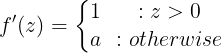
where 0 <  < 1
< 1
Traditional ReLU units by design do not propagate any error for non-positive z – the leaky ReLU modifies this such that a small error is allowed to propagate backwards even when z is negative:
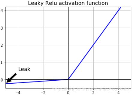
- 解决了RELU死神经元的问题 : 替换Relu左边水平线的主要优点是去除零梯度。在这种情况下,上图左边的梯度是非零的,所以该区域的神经元不会成为死神经元。
- The hyperparameter defines how much the function “leaks”泄漏: it is the slope of the function for
 and is typically set to 0.01. This small slope ensures that leaky ReLUs never die; they can go into a long coma怠惰/昏迷, but they have a chance to eventually wake up. A 2015 paper compared several variants of the ReLU activation function, and one of its conclusions was that the leaky variants always outperformed the strict ReLU activation function. In fact, setting
  (a huge leak) seemed to result in better performance than
  (a small leak).
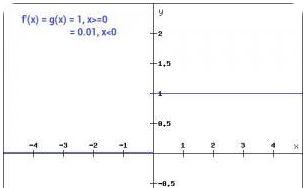
PRelu ###############
![]()
For backpropagation, its gradient is 
- if
 ,
,  becomes ReLU
 - if
 , becomes leaky ReLU
 - if
 is a learnable parameter, becomes PReLU
 -
如果神经网络中出现死神经元,那么PReLU函数就是最好的选择。
- PReLU was reported to strongly outperform ReLU on large image datasets, but on smaller datasets it runs the risk of overfitting the training set.
- 在PReLU函数中, 也是可训练的函数。神经网络还会学习的价值,以获得更快更好的收敛。 is authorized to be learned during training (instead of being a hyperparameter, it becomes a parameter that can be modified by backpropagation like any other parameter)。 当Leaky ReLU函数仍然无法解决死神经元问题并且相关信息没有成功传递到下一层时,可以考虑使用PReLU函数。
ELU( Exponential Linear Unit ) ###############
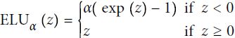

-
Exponential Linear Unit (ELU) that outperformed all the ReLU variants in the authors’ experiments: training time was reduced, and the neural network performed better on the test set.
The ELU activation function looks a lot like the ReLU function, with a few major differences:-
It takes on negative values when z < 0, which allows the unit to have an average output closer to 0 and helps alleviate the vanishing gradients problem. The hyperparameter α defines the value that the ELU function approaches when z is a large negative number 超参数 α 定义了当 z 是一个大的负数时 ELU 函数接近的值. It is usually set to 1### elu(z,1) ###, but you can tweak it like any other hyperparameter.
-
It has a nonzero gradient for z < 0, which avoids the dead neurons problem.
-
If α is equal to 1 then the function is smooth everywhere, including around z = 0, which helps speed up Gradient Descent since it does not bounce弹回 as much to the left and right of z = 0.
-
缺点:The main drawback of the ELU activation function is that it is slower to compute than the ReLU function and its variants (due to the use of the exponential function). Its faster convergence rate during training compensates for that slow computation, but still, at test time an ELU network will be slower than a ReLU network.
-
SELU (Scaled ELU):###############
Scaled ELU (SELU) activation function is a scaled variant of the ELU activation function. if you build a neural network composed exclusively of a stack of dense layers仅由一叠dense layers组成, and if all hidden layers use the SELU activation function, then the network will self-normalize: the output of each layer will tend to preserve a mean of 0 and standard deviation of 1 during training, which solves the vanishing/exploding gradients problem. As a result, the SELU activation function often significantly outperforms other activation functions for such neural nets (especially deep ones). There are, however, a few conditions for self-normalization to happen (see the paper for the mathematical justification):
- The input features must be standardized (mean 0 and standard deviation 1).
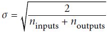
- Every hidden layer’s weights must be initialized with LeCun normal initialization. In Keras, this means setting kernel_initializer="lecun_normal".
( Xavier(Glorot) initialization (when using the logistic activation function)
Normal distribution with mean 0 and standard deviation
 OR
OR 
where and
and  are the number of input and output connections for the layer whose weights are being initialized (also called fan-in and fan-out;
 ).
).
Or a uniform distribution between ‐r and +r, with
 OR
OR 
LeCun initialization is equivalent to Glorot initialization when
- The network’s architecture must be sequential.
Unfortunately, if you try to use SELU in nonsequential architectures, such as recurrent networks (see https://blog.csdn.net/Linli522362242/article/details/114941730) or networks with skip connections (i.e., connections that skip layers, such as in Wide & Deep nets), self-normalization will not be guaranteed, so SELU will not necessarily outperform other activation functions. - The paper only guarantees self-normalization if all layers are dense, but some researchers have noted that the SELU activation function can improve performance in convolutional neural nets as well (see https://blog.csdn.net/Linli522362242/article/details/108302266).
Softplus:###############
![]() OR softplus(x) = log(exp(x) + 1)
OR softplus(x) = log(exp(x) + 1)![]()

Soft sign:###############
The soft sign function is another nonlinearity which can be considered an alternative to tanh since it too does not saturate as easily as hard tanh clipped functions:![]() and
and ![]()
where sgn is the signnum function which returns ±1 depending on the sign of z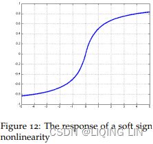
#############################For example, a rectified linear unit (ReLU) function is written as: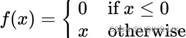 OR
OR
The ReLU activates a node with the same input value only when the input is above zero. Researchers prefer to use ReLU as it trains better than sigmoid activation functions![]() . We will be using ReLU in later parts of this chapter.
. We will be using ReLU in later parts of this chapter.
In another example, the leaky ReLU is written as: 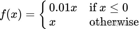 OR
OR![]()
The leaky ReLU addresses the issue of a dead ReLU(解决了RELU死神经元的问题) when by having a small negative slope around 0.01 when ![]() .
.
Loss functions
(MAE, MSE, Huber, Logistic,Cross entropy, Focal, Hinge, Exponential,Softmax, Quantile)
The loss function computes the error between the predicted value of a model and the actual value. The smaller the error value, the better the model is in prediction. Some loss functions used in regression-based models are:
Mean Absolute Error (MAE) loss:###############
 OR
OR
 are the predicted and
  actual value.
The mean squared error might penalize large errors too much and cause your model to be imprecise.
Mean Squared Error (MSE) loss:###############
 OR
OR 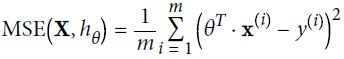
The mean absolute error would not penalize outliers as much, but training might take a while to converge, and the trained model might not be very precise.
The term  which in the following equation that is just added for our convenience, which will make it easier to derive the gradient
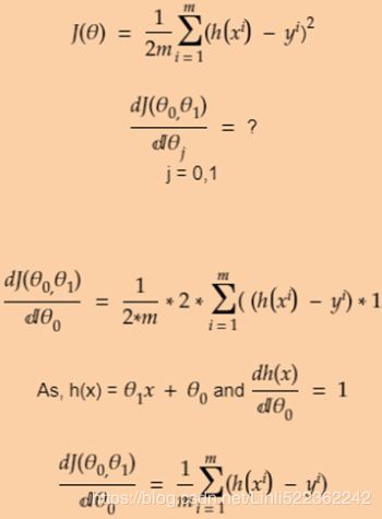
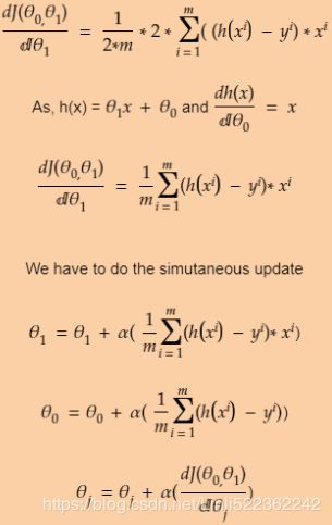
Note: multiply the gradient vector by alpha  to determine the size of the downhill step(learning rate
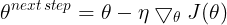 ) :
) : 
right ![]() is for next step (downhill step), left
is for next step (downhill step), left ![]() is currently theta value; Once the left
is currently theta value; Once the left ![]() == right
== right ![]() , h(x) ==y means the gradient
, h(x) ==y means the gradient  equal to 0.
Huber loss :###############
https://www.cnblogs.com/nowgood/p/Huber-Loss.html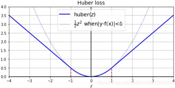
 OR
OR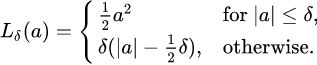
The Huber loss is quadratic ![]() when the error is smaller than a threshold
when the error is smaller than a threshold  (typically 1) but linear
![]() when the error is larger than . The linear part makes it less sensitive to outliers than the Mean Squared Error, and the quadratic part allows it to converge faster and be more precise than the Mean Absolute Error) instead of the good old MSE.
when the error is larger than . The linear part makes it less sensitive to outliers than the Mean Squared Error, and the quadratic part allows it to converge faster and be more precise than the Mean Absolute Error) instead of the good old MSE.
Quantile loss :###############
Given a prediction ![]() and outcome , the mean regression loss for a quantile
and outcome , the mean regression loss for a quantile ![]() is
is![]()
For a set of predictions, the loss will be its average.
https://towardsdatascience.com/regression-prediction-intervals-with-xgboost-428e0a018b https://www.wikiwand.com/en/Quantile_regression
In the regression loss equation above, as ![]() has a value between 0 and 1, the first term will be positive and dominate when under-predicting,
has a value between 0 and 1, the first term will be positive and dominate when under-predicting, ![]() , and the second term will dominate when over-predicting,
, and the second term will dominate when over-predicting, ![]() .
.
For ![]() equal to 0.5, under-prediction and over-prediction will be penalized by the same factor, and the median is obtained.
equal to 0.5, under-prediction and over-prediction will be penalized by the same factor, and the median is obtained.
The larger the value of ![]() , the more under-predictions are penalized compared to over-predictions.
, the more under-predictions are penalized compared to over-predictions.
For ![]() equal to 0.75, under-predictions will be penalized by a factor of 0.75, and over-predictions by a factor of 0.25. The model will then try to avoid under-predictions approximately three times as hard as over-predictions, and the 0.75 quantile will be obtained.
equal to 0.75, under-predictions will be penalized by a factor of 0.75, and over-predictions by a factor of 0.25. The model will then try to avoid under-predictions approximately three times as hard as over-predictions, and the 0.75 quantile will be obtained.
def quantile_loss(q, y, y_p):
        e = y-y_p
        return tf.keras.backend.mean( tf.keras.backend.maximum( q*e,
                                                                (q-1)*e
                                                              )
                                    )
https://www.evergreeninnovations.co/blog-quantile-loss-function-for-machine-learning/
As the name suggests, the quantile regression loss function is applied to predict quantiles. A quantile is the value below which a fraction of observations in a group falls. For example, a prediction for quantile 0.9 should over-predict 90% of the times.
https://www.wikiwand.com/en/Quantile_regression
Some loss functions used in classification-based models are:
Logistic loss:###############
Minimize:
https://blog.csdn.net/Linli522362242/article/details/126672904
Minimize MSE:  OR and
  is 0 or 1,
 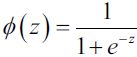 ==>
==> OR
OR 
==>  is the index of current sample
For Minimize MSE:
if  =1 or
=1 or  , Maximize
  for closing to 1, and
 ![]() =1 ==>Maximize
=1 ==>Maximize![]() for closing to 1
for closing to 1
if =0 or  , Minimize for closing to 0, then
 ![]() =1 ==>Maximize
=1 ==>Maximize![]() for closing to 1
for closing to 1
==>Convert to Maximize the likelihood , (y=0, 1)
==>Use logarithm to convert multiplication to addition:
==>Minimize log-likelihood:
OR 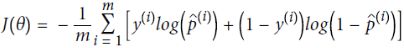
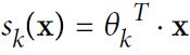
- Equation 4-19. Softmax score for class k
Note that each class has its own dedicated parameter vector
Equation 4-20. Softmax function
K is the number of classes
s(x) is a vector containing the scores of each class for the instance x. is the estimated probability
 that the instance x belongs to class k given the scores of each class for that instance.
Cross entropy cost function :###############
Minimize 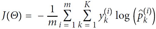 Equation 4-22
 is equal to 1 if the target class for the th instance is
  ; otherwise, it is equal to 0.
Notice that when there are just two classes (K = 2), this cost function is equivalent to the Logistic Regression’s cost function (log loss; see Equation 4-17
let’s take a look at training. The objective is to have a model that estimates a high probability for the target class (and consequently a low probability for the other classes). Minimizing the cost function shown in Equation 4-22, called the cross entropy交叉熵, should lead to this objective because it penalizes the model when it estimates a low probability(to have high cost function) for a target class. Cross entropy is frequently used to measure how well a set of estimated class probabilities match the target classes. lower x higher cost(
![]() )
)
Let’s say, Foreground (Let’s call it class 1) is correctly classified with p=0.95
CE(FG) = -ln (0.95) =0.05
And background (Let’s call it class 0) is correctly classified with p=0.05
CE(BG)=-ln (1- 0.05) =0.05
The problem is, with the class imbalanced dataset, when these small losses are sum over the entire images can overwhelm the overall loss (total loss). And thus, it leads to degenerated models.
weighted(![]() ) Cross entroy cost function:
) Cross entroy cost function: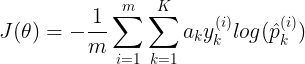
但是,当我们处理大量负样本![]() 、少量正样本
、少量正样本![]() 的情况时(e g 50000:20),即使我们把负样本的权重设置的很低,但是因为负样本的数量太多,积少成多,负样本的损失函数也会主导损失函数
的情况时(e g 50000:20),即使我们把负样本的权重设置的很低,但是因为负样本的数量太多,积少成多,负样本的损失函数也会主导损失函数
Let’s say, Foreground (Let’s call it class 1) is correctly classified with p=0.95
CE(FG) = -0.25*ln (0.95) =0.0128
And background (Let’s call it class 0) correctly classified with p=0.05
CE(BG)=-(1-0.25) * ln (1- 0.05) =0.038
While it does a good job differentiating positive & negative classes correctly but still does not differentiate between easy/hard examples.
And that’s where Focal loss (extension to cross-entropy) comes to rescue.
Focal loss:###############
Focal loss is just an extension of the cross-entropy loss function that would down-weight easy examples and focus training on hard negatives.focal loss 是一种处理样本分类不均衡的损失函数,它侧重的点是根据样本分辨的难易程度给样本对应的损失添加权重,即给容易区分的样本添加较小的权重![]() , 给难分辨的样本添加较大的权重,
, 给难分辨的样本添加较大的权重, ![]() 那么,损失函数的可以写为:
那么,损失函数的可以写为:![]()
因为 ![]() ,那么上述的损失函数中
,那么上述的损失函数中![]() 主导损失函数,也就是将损失函数的重点集中于难分辨的样本上,对应损失函数的名称:focal loss。
主导损失函数,也就是将损失函数的重点集中于难分辨的样本上,对应损失函数的名称:focal loss。![]()
通常将分类置信度接近1或接近0的样本称为易分辨样本( ![]() 越大 or
越大 or ![]() 越大,说明分类的置信度越高,代表样本越易分),其余的称之为难分辨样本。换句话说,也就是我们有把握确认属性的样本称为易分辨样本,没有把握确认属性的样本称之为难分辨样本。
越大,说明分类的置信度越高,代表样本越易分),其余的称之为难分辨样本。换句话说,也就是我们有把握确认属性的样本称为易分辨样本,没有把握确认属性的样本称之为难分辨样本。
比如在一张图片中,我们获得是人的置信度为0.9,那么我们很有把握它是人,所以此时认定该样本为易分辨样本。同样,获得是人的置信度为0.6,那么我们没有把握它是人,所以称该样本为难分辨样本。
As you can see, the blue line(![]() ) in the below diagram, when
) in the below diagram, when ![]() is very close to 1 (when class_label y_k=1) or 0 (when class_label y_k = 0), easily classified examples with large
is very close to 1 (when class_label y_k=1) or 0 (when class_label y_k = 0), easily classified examples with large ![]() can incur a loss with non-trivial重大 magnitude.可以从图中发现,那些即使置信度很高的样本在标准交叉熵里也会存在重大损失。而且在实际中,置信度很高的负样本
can incur a loss with non-trivial重大 magnitude.可以从图中发现,那些即使置信度很高的样本在标准交叉熵里也会存在重大损失。而且在实际中,置信度很高的负样本![]() 往往占总样本的绝大部分,如果将这部分损失去除或者减弱,那么损失函数的效率会更高。
往往占总样本的绝大部分,如果将这部分损失去除或者减弱,那么损失函数的效率会更高。
We shall note the following properties of the focal loss:
- When an example is misclassified and
 is small(→ 0), the modulating factor
 is near 1 and the loss is almost unaffected.
 - As → 1, the factor goes to 0 and the loss for well-classified examples is down weighed
 .
. - The focusing parameter γ>0 smoothly adjusts the rate at which easy examples are down-weighted.
As is increased, the effect of modulating factor is likewise increased. (After a lot of experiments and trials, researchers have found γ = 2 to work best)
Intuitively, the modulating factor
when γ =0, FL is equivalent to CEreduces the loss contribution from easy examples(higher confidence in the classification) and extends the range in which an example receives the low loss.
https://www.analyticsvidhya.com/blog/2020/08/a-beginners-guide-to-focal-loss-in-object-detection/#:~:text=In%20simple%20words%2C%20Focal%20Loss,to%20down%2Dweight%20easy%20examples%20(
Hinge loss:###############
对线性SVM分类器来说,方法之一是使用梯度下降,使从原始问题导出的cost function最小化。线性SVM分类器cost function成本函数:
成本函数中的第一项会推动模型得到一个较小的权重向量w,从而使间隔更大.
(
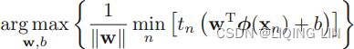 ==>At first,
 (to find the closest of data points to decision boundary
![]() ),Then maximize
),Then maximize for maximizing the margin( to choose the decision boundary or to find the support vectors
 OR
OR that determine the location boundary) ==> (maximize ==>
 is equivalent to minimizing
  )==>
)==> 
)
第二项则计算全部的间隔违例。如果没有一个示例位于街道之上,并且都在街道正确的一边,那么这个实例的间隔违例为0;如不然,则该实例的违例大小与其到街道正确一边的距离成正比。所以将这个项最小化,能够保证模型使间隔违例尽可能小,也尽可能少。
函数被称为hinge损失函数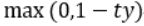 (如下图所示)。其中,t为目标值 class label(-1或+1),y是分类器输出的预测值 ,并不直接是类标签。其含义为,
当t和y的符号相同时(表示y预测正确)并且|y|≥1时,hinge loss为0 ( since max(0, 1-ty<0) );当t和y的符号相反时,hinge loss随着y的增大线性增大(since max(0, 1-ty>0)==> 1-ty)。
Hinge loss用于最大间隔(maximum-margin)分类,其中最有代表性的就是支持向量机SVM。
Hinge函数的标准形式: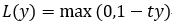
(与上面统一的形式: )
)
Exponential loss:###############
![]() where y is the expected output(actual class label, either 1 or -1) and f(x) is the model output(prediction) given the feature x.
where y is the expected output(actual class label, either 1 or -1) and f(x) is the model output(prediction) given the feature x. 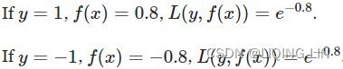
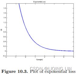
The exponential loss is convex and grows exponentially for negative values which makes it more sensitive to outliers. The exponential loss is used in the AdaBoost algorithm. The principal attraction of exponential loss in the context of additive modeling is computational. The additive expansion produced by AdaBoost is estimating onehalf of the log-odds of P(Y = 1|x). This justifies using its sign as the classification rule.https://yuan-du.com/post/2020-12-13-loss-functions/decision-theory/
Optimizers
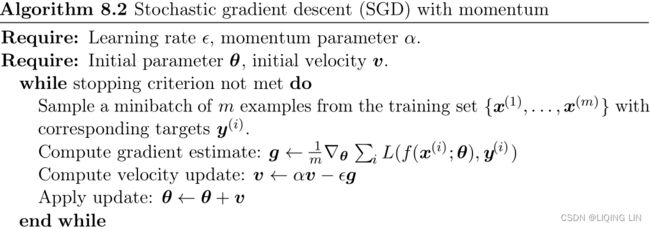
(Gradient Descent, SGD, Momentum, NAG, AdaGrad, RMSprop, Adam, AdaMax, Nadam, Adadelta,)
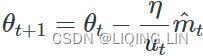
Optimizers help to tweak the model weights(θ ← θ –  , for example
  ) optimally in minimizing the loss function. There are several types of optimizers that you may come across in deep learning:
Gradient Descent : ###############
These two facts have a great consequence: Gradient Descent is guaranteed to approach arbitrarily close the global minimum The general idea of Gradient Descent is to tweak parameters iteratively in order to minimize a cost function.
It does not care about what the earlier gradients were. If the local gradient is tiny, it goes very slowly. Concretely, you start by filling θ with random values (this is called random initialization), and then you improve it gradually, taking one baby step at a time, each step attempting to decrease the cost function (e.g., the MSE), until the algorithm converges to a minimum(see Figure 4-3)
 An important parameter in Gradient Descent is the size of the steps, determined by the learning rate hyperparameter
![]() . If the learning rate is too small, then the algorithm will have to go through many iterations to converge, which will take a long time (see Figure 4-4).
. If the learning rate is too small, then the algorithm will have to go through many iterations to converge, which will take a long time (see Figure 4-4). On the other hand, if the learning rate is too high, you might jump across the valley and end up on the other side, possibly even higher up than you were before. This might make the algorithm diverge, with larger and larger values, failing to find a good solution (see Figure 4-5).
 Finally, not all cost functions look like nice regular bowls. There may be holes洞, ridges山脊, plateaus 高原, and all sorts of irregular terrains地形, making convergence to the minimum very difficult. Figure 4-6 shows the two main challenges with Gradient Descent: if the random initialization starts the algorithm on the left, then it will converge to a local minimum, which is not as good as the global minimum. If it starts on the right, then it will take a very long time to cross the plateau, and if you stop too early you will never reach the global minimum.
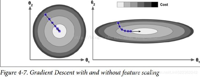
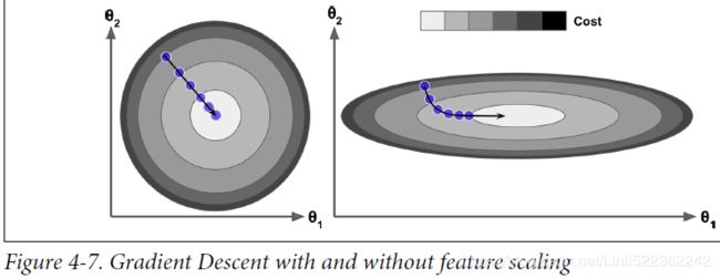 In fact, the cost function has the shape of a bowl, but it can be an elongated被延长 bowl if the features have very different scales. Figure 4-7 shows Gradient Descent on a training set where features 1 and 2 have the same scale (on the left), and on a training set where feature 1 has much smaller values than feature 2 (on the right).Since feature 1 is smaller, it takes a larger change in θ1 to affect the cost function, which is why the bowl is elongated along the θ1 axis.
As you can see, on the left the Gradient Descent algorithm goes straight toward the minimum, thereby reaching it quickly, whereas on the right it first goes in a direction almost orthogonal to the direction of the global minimum, and it ends with a long
march down an almost flat valley. It will eventually reach the minimum, but it will take a long time.
#########################
WARNING
When using Gradient Descent, you should ensure that all features have a similar scale (e.g., using Scikit-Learn’s StandardScaler class), or else it will take much longer to converge.
#########################
SGD (Stochastic Gradient Descent) :###############
https://blog.csdn.net/Linli522362242/article/details/104005906
The main problem with Batch Gradient Descent is the fact that it uses the whole training set to compute the gradients at every step, which makes it very slow when the training set is large. At the opposite extreme, Stochastic Gradient Descent just picks a random instance in the training set at every step and computes the gradients based only on that single instance. Obviously this makes the algorithm much faster since it has very little data to manipulate at every iteration. It also makes it possible to train on huge training sets, since only one instance needs to be in memory at each iteration (SGD can be implemented as an out-of-core algorithm.)
On the other hand, due to its stochastic (i.e., random) nature, this algorithm is much less regular than Batch Gradient Descent: instead of gently decreasing平缓的下降 until it reaches the minimum, the cost function will bounce跳 up and down, decreasing only on average大体上. Over time it will end up very close to the minimum, but once it gets there it will continue to bounce around, never settling down (see Figure 4-9). So once the algorithm stops, ![]() the final parameter values are good, but not optimal.
the final parameter values are good, but not optimal.![]()
 When the cost function is very irregular (as in the left figure), this can actually help the algorithm jump out of local minima, so Stochastic Gradient Descent has a better chance of finding the global minimum than Batch Gradient Descent does.
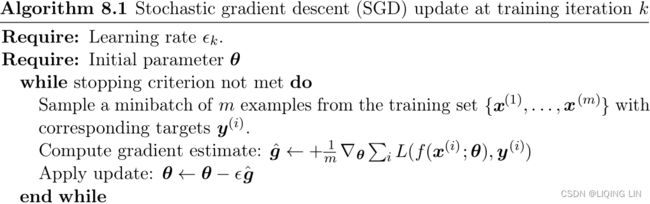
Therefore randomness is good to escape from local optima, but bad because it means that the algorithm can never settle at the minimum. One solution to this dilemma/dɪˈlemə/窘境is to gradually reduce the learning rate. The steps start out large (which helps make quick progress and escape local minima), then get smaller and smaller, allowing the algorithm to settle at the global minimum. This process is called simulated annealing/əˈniːlɪŋ/模拟退火, because it resembles类似于 the process of annealing in metallurgy冶金 where molten熔融 metal is slowly cooled down. The function that determines the learning rate at each iteration is called the learning schedule. If the learning rate is reduced too quickly, you may get stuck in a local minimum, or even end up frozen halfway to the minimum. If the learning rate is reduced too slowly, you may jump around the minimum for a long time and end up with a suboptimal solution if you halt training too early.
#################################
Note
In stochastic gradient descent implementations, the fixed learning rate ![]() is often replaced by an adaptive learning rate that decreases over time, for example,
is often replaced by an adaptive learning rate that decreases over time, for example, where
where  and
and  are constants. Note that stochastic gradient descent does not reach the global minimum but an area very close to it. By using an adaptive learning rate, we can achieve further annealing磨炼 to a better global minimum
#################################
theta_path_sgd = []
m=len(X_b)
np.random.seed(42)

n_epochs = 50
t0,t1= 5,50

def learning_schedule(t):
    return t0/(t+t1)

theta = np.random.randn(2,1)

for epoch in range(n_epochs): # n_epochs=50 replaces n_iterations=1000
    for i in range(m): # m = len(X_b)
        if epoch==0 and i<20:
            y_predict = X_new_b.dot(theta)
            style="b-" if i>0 else "r--"
            plt.plot(X_new,y_predict, style)######

        random_index = np.random.randint(m)  ##### Stochastic
        xi = X_b[random_index:random_index+1]
        yi = y[random_index:random_index+1]
        gradients = 2*xi.T.dot( xi.dot(theta) - yi ) ##### Gradient
        eta=learning_schedule(epoch*m + i) ############## e.g. 5/( (epoch*m+i)+50)
        theta = theta-eta * gradients  ###### Descent
        theta_path_sgd.append(theta)


plt.plot(X, y, "b.")
plt.xlabel("$x_1$", fontsize=18)
plt.ylabel("$y$", rotation=0, fontsize=18)
plt.title("Figure 4-10. Stochastic Gradient Descent first 10 steps")

plt.axis([0,2, 0,15])
plt.show()
https://blog.csdn.net/Linli522362242/article/details/104005906 04_TrainingModels_Normal Equation(正态方程,正规方程) Derivation_Gradient Descent_Polynomial Regression_LIQING LIN的博客-CSDN博客
Momentum:###############
 # it subtracts the local gradient * η from the momentum vector m, m is negative
 # it updates the weights by adding this momentum vector m, note m is negative OR
#* 下降初期时,使用上一次参数更新,下降方向一致,乘上较大的β能够进行很好的加速
#* 下降中后期时,在局部最小值来回震荡的时候, -->0,β使得更新幅度增大,跳出陷阱
#* 在梯度改变方向的时候(梯度上升,梯度方向与βm相反),能够减少更新总而言之,momentum项能够在相关方向加速SGD,抑制振荡,从而加快收敛
The momentum term (βm) increases for dimensions whose gradients point in the same directions and reduces updates for dimensions whose gradients change directions. As a result, we gain faster convergence and reduced oscillation.
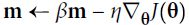
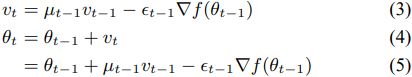
Momentum optimization cares a great deal about what previous gradients were: at each iteration, it subtracts the local gradient from the momentum vector m (multiplied by the learning rate η), and it updates the weights by adding this momentum vector m (see Equation 11-4). In other words, the gradient is used for acceleration, not for speed. To simulate some sort of friction摩擦 mechanism and prevent the momentum m from growing too large, the algorithm introduces a new hyperparameter β, called the momentum, which must be set between 0 (high friction) and 1 (no friction). A typical momentum value is 0.9.
You can easily verify that if the gradient remains constant, the terminal velocity m (i.e., the maximum size of the weight updates) is equal to that gradient multiplied by the learning rate η multiplied by 1/(1–β) (ignoring the sign).### VS and 0<= β <1
It is thus helpful to think of the momentum hyperparameter β in terms of 
 For example, if β = 0.9, then the terminal velocity is equal to 10 times the gradient times the learning rate, so momentum optimization ends up going 10 times faster than Gradient Descent! This allows momentum optimization to escape from plateaus停滞时期 much faster than Gradient Descent. We saw in Chapter 4 that when the inputs have very different scales, the cost function will look like an elongated bowl (see Figure 4-7). Gradient Descent goes down the steep slope陡坡 quite fast, but then it takes a very long time to go down the valley深谷. In contrast, momentum optimization will roll down the valley faster and faster until it reaches the bottom (the optimum). In deep neural networks that don’t use Batch Normalization, the upper layers will often end up having inputs with very different scales, so using momentum optimization helps a lot. It can also help roll past local optima.
Due to the momentum, the optimizer may overshoot超调 a bit, then come back, overshoot again, and oscillate[ˈɑsɪleɪt]使振荡 like this many times before stabilizing at the minimum. This is one of the reasons it’s good to have a bit of friction in the system(β): it gets rid of these oscillations and thus speeds up convergence.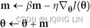 OR
OR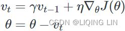
class MomentumGradientDescent(MiniBatchGradientDescent):
    def __init__(self, gamma=0.9, **kwargs):
        self.gamma = gamma  # gammar also called momentum, 当gamma=0时,相当于小批量随机梯度下降
        super(MomentumGradientDescent, self).__init__(**kwargs)

    def fit(self, X, y):
        X = np.c_[np.ones(len(X)), X]
        n_samples, n_features = X.shape

        self.theta = np.ones(n_features)
        self.velocity = np.zeros_like(self.theta) ################
        self.loss_ = [0]

        self.i = 0
        while self.i < self.n_iter:#n_iter: epochs
            self.i += 1
            if self.shuffle:
                X, y = self._shuffle(X, y)

            errors = []
            for j in range(0, n_samples, self.batch_size):
                mini_X, mini_y = X[j: j + self.batch_size], y[j: j + self.batch_size]
                error = mini_X.dot(self.theta) - mini_y
                errors.append(error.dot(error))
                mini_gradient = 1/ self.batch_size * mini_X.T.dot(error)# without*2 since cost/loss
                self.velocity = self.velocity * self.gamma + self.eta * mini_gradient
                self.theta -= self.velocity
                                                      #loss*1/2 for convenient computing gradient
            loss = 1 / (2 * self.batch_size) * np.mean(errors)
            delta_loss = loss - self.loss_[-1] #当结果改善的变动低于某个阈值时,程序提前终止
            self.loss_.append(loss)
            if np.abs(delta_loss) < self.tolerance:
                break
        return self
In keras:
tf.keras.optimizers.SGD(
    learning_rate=0.01, momentum=0.0, nesterov=False, name="SGD", **kwargs
)
* The update rule for θ with gradient g when momentum(β) is 0.0:

* The update rule when momentum is larger than 0.0(β>0):
the initial ![]() ,
, ![]() ==>
==> 
Note : ![]() :
:
![]() 有方向 -gradent 是向下(negative)==>
有方向 -gradent 是向下(negative)==> ![]()
![]() # note usually initialize
# note usually initialize ![]()
![]() :
:
![]()
![]()
https://github.com/tensorflow/tensorflow/blob/v1.15.0/tensorflow/python/keras/optimizer_v2/gradient_descent.py#L29-L164
if `nesterov` is False, gradient is evaluated at theta(t).
# v(t+1) = momentum * v(t) - learning_rate * gradient
# theta(t+1) = theta(t) + v(t+1)

velocity = momentum * velocity - learning_rate * g
w = w + velocity
OR keras
# https://github.com/tensorflow/tensorflow/blob/v2.2.0/tensorflow/python/keras/optimizers.py
#
class SGD(Optimizer):
  """Stochastic gradient descent optimizer.
  Includes support for momentum,
  learning rate decay, and Nesterov momentum.
  Arguments:
      lr: float >= 0. Learning rate.
      momentum: float >= 0. Parameter that accelerates SGD in the relevant
        direction and dampens oscillations.
      decay: float >= 0. Learning rate decay over each update.
      nesterov: boolean. Whether to apply Nesterov momentum.
  """

  def __init__(self, lr=0.01, momentum=0., decay=0., nesterov=False, **kwargs):
    super(SGD, self).__init__(**kwargs)
    with K.name_scope(self.__class__.__name__):
      self.iterations = K.variable(0, dtype='int64', name='iterations')
      self.lr = K.variable(lr, name='lr')
      self.momentum = K.variable(momentum, name='momentum')
      self.decay = K.variable(decay, name='decay')
    self.initial_decay = decay
    self.nesterov = nesterov

  def _create_all_weights(self, params):
    shapes = [K.int_shape(p) for p in params]
    moments = [K.zeros(shape) for shape in shapes] ##########################
    self.weights = [self.iterations] + moments
    return moments

  def get_updates(self, loss, params):
    grads = self.get_gradients(loss, params)
    self.updates = [state_ops.assign_add(self.iterations, 1)]

    lr = self.lr
    if self.initial_decay > 0:
      lr = lr * (  # pylint: disable=g-no-augmented-assignment
          1. /
          (1. +
           self.decay * math_ops.cast(self.iterations, K.dtype(self.decay))))
    # momentum
    moments = self._create_all_weights(params)
    for p, g, m in zip(params, grads, moments):
      v = self.momentum * m - lr * g  # velocity # m=0 ==> v = - lr * g #####
      self.updates.append(state_ops.assign(m, v))

      if self.nesterov:
        new_p = p + self.momentum * v - lr * g
      else:
        new_p = p + v ############################ SGD with momentum ########

      # Apply constraints.
      if getattr(p, 'constraint', None) is not None:
        new_p = p.constraint(new_p)

      self.updates.append(state_ops.assign(p, new_p))
    return self.updates
When nesterov=True, this rule becomes: # velocity m < 0
if `nesterov` is True, gradient is evaluated at theta(t) + momentum * v(t),
and the variables always store theta + m v instead of theta
# do the momentum stage first for gradient descent part
velocity = momentum * velocity - learning_rate * g # for gradient descent part
# update the parameters ==> then do the gradient descent part ==> update weight
w = w + momentum * velocity - learning_rate * g # g:evaluated at theta(t)+momentum*v(t)Nesterov Accelerated Gradient( NAG ) :###############


the initial ![]() ,
, ![]() ==>
==> ![]()
Note : ![]() :
:
![]() 无方向 gradent >0 ==>
无方向 gradent >0 ==> ![]()
![]() # note usually initialize
# note usually initialize ![]()
#OR random_uniform(shape=[n_features,1],minval=-1.0, maxval=1.0,)
![]() :
:
![]()
![]()
#######Nesterov Accelerated Gradient and Momentum![]() http://proceedings.mlr.press/v28/sutskever13.pdf
http://proceedings.mlr.press/v28/sutskever13.pdf
the initial ![]() ,
, ![]() ==>
==> ![]()
Note : ![]() :
:
![]() 有方向 -gradent 是向下(negative)==>
有方向 -gradent 是向下(negative)==> ![]()
![]() # note usually initialize
# note usually initialize ![]()
#OR random_uniform(shape=[n_features,1],minval=-1.0, maxval=1.0,)
![]() :
:
![]()
![]()
class NesterovAccelerateGradient(MomentumGradientDescent):
    def __init__(self, **kwargs):
        super(NesterovAccelerateGradient, self).__init__(**kwargs)

    def fit(self, X, y):
        X = np.c_[np.ones(len(X)), X]
        n_samples, n_features = X.shape #n_features: n_features+1

        #OR random_uniform(shape=[n_features,1],minval=-1.0, maxval=1.0,)
        self.theta = np.ones(n_features)
        self.velocity = np.zeros_like(self.theta)#################
        self.loss_ = [0]

        self.i = 0
        while self.i < self.n_iter:
            self.i += 1
            if self.shuffle:
                X, y = self._shuffle(X, y)

            errors = []
            for j in range(0, n_samples, self.batch_size):
                mini_X, mini_y = X[j: j + self.batch_size], y[j: j + self.batch_size]

                # gamma also called momentum  '-' since we use -self.velocity
                error = mini_X.dot(self.theta - self.gamma * self.velocity) - mini_y############
                errors.append(error.dot(error))
                mini_gradient = 1 / self.batch_size * mini_X.T.dot(error)

                self.velocity = self.velocity * self.gamma + self.eta * mini_gradient
                self.theta -= self.velocity
            loss = 1 / (2 * self.batch_size) * np.mean(errors)
            delta_loss = loss - self.loss_[-1]
            self.loss_.append(loss)
            if np.abs(delta_loss) < self.tolerance:
                break
        return self
in keras:
if `nesterov` is True, gradient is evaluated at theta(t) + momentum * v(t),
and the variables always store theta + m v instead of theta
# do the momentum stage first for gradient descent part
velocity = momentum * velocity - learning_rate * g # for gradient descent part
# update the parameters ==> then do the gradient descent part ==> update weight
w = w + momentum * velocity - learning_rate * g
#######
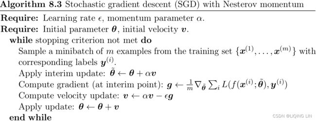
Nesterov momentum optimization measures the gradient of the cost function not at the local position θ(![]() ) but slightly ahead in the direction of the momentum, at θ + βm (
) but slightly ahead in the direction of the momentum, at θ + βm (![]() ).
).
This small tweak works because in general the momentum vector m will be pointing in the right direction (i.e., toward the optimum), so it will be slightly more accurate to use the gradient measured a bit farther in that direction![]() rather than using the gradient at the original position
rather than using the gradient at the original position![]() , as you can see in Figure 11-6 (where
, as you can see in Figure 11-6 (where  represents the gradient of the cost function measured at the starting point θ, and
  represents the gradient at the point located at θ + βm,
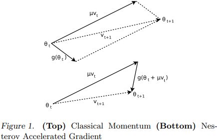
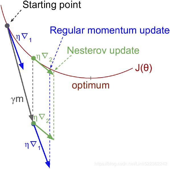
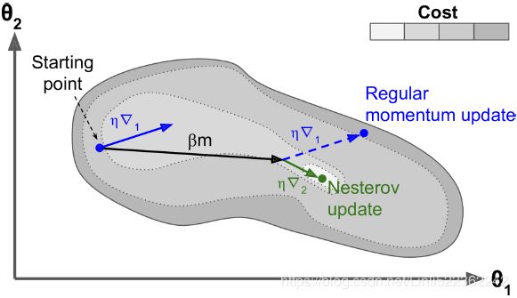
Figure 11-6. Regular versus Nesterov Momentum optimization( ==β); the former applies the gradients computed before the momentum step(βm), while the latter applies the gradients######
 computed after.
While Momentum first computes the current gradient (blue vector) and then takes a big jump(red vector,βm) in the direction of the updated accumulated gradient,
NAG first makes a big jump in the direction of the previous accumulated gradient (red vector,βm), measures the gradient (green vector) and then makes a correction, which results in the complete NAG update. This anticipatory update prevents us from going too fast and results in increased responsiveness, which has significantly increased the performance of RNNs on a number of tasks.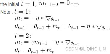 <==
<==
As you can see, the Nesterov update ends up slightly closer to the optimum. After a while, these small improvements add up and NAG ends up being significantly faster than regular Momentum optimization. Moreover, note that when the momentum βm pushes the weights across a valley, continues to push further across the valley, while pushes back toward the bottom of the valley(更正方向). This helps reduce oscillations and thus converges faster.
https://blog.csdn.net/Linli522362242/article/details/106982127
keras Nesterov Accelerated Gradient( NAG )
################### ###################
 OR
OR![]()
where ![]() are the model parameters,
are the model parameters, ![]() the velocity,
the velocity, ![]() ∈ [0, 1] the momentum (decay) coefficient and
∈ [0, 1] the momentum (decay) coefficient and ![]() > 0 the learning rate at iteration
> 0 the learning rate at iteration ![]() , f(θ) is the objective function and
, f(θ) is the objective function and ![]() is a shorthand notation for the gradient
is a shorthand notation for the gradient ![]() . These equations have a form similar to standard momentum updates: note
. These equations have a form similar to standard momentum updates: note ![]()
 OR
OR
and differ only in the evaluation point of the gradient at each iteration. This important difference, thought to counterbalance too high velocities ![]() by “peeking ahead” actual objective values
by “peeking ahead” actual objective values![]() (更正方向) in the candidate search direction, results in significantly improved RNN performance on a number of tasks.
(更正方向) in the candidate search direction, results in significantly improved RNN performance on a number of tasks.
In this section, we derive a new formulation of Nesterov momentum differing from (3) and (5) only in the linear combination coefficients of the velocity and gradient contributions at each iteration, and we offer an alternative interpretation of the method. The key departure from (1) and (2) resides in committing to the “peekedahead” parameters ![]() and backtracking by the same amount before each update. Our new parameters
and backtracking by the same amount before each update. Our new parameters ![]() updates become:
updates become:![]()
![]() (6)==>keras fomula
(6)==>keras fomula![]()
![]()
![]()
![]()
![]()
![]() ==>keras
==>keras ![]()
![]()
![]() (7)
(7)
Assuming a zero initial velocity ![]() = 0 and velocity at convergence of optimization
= 0 and velocity at convergence of optimization ![]() ≃ 0 (since
≃ 0 (since ![]() ), the parameters
), the parameters  are a completely equivalent replacement of θ.
Note that equation (7) is identical to regular/classical momentum (5) with different linear combination coefficients. More precisely, for an equivalent velocity update (6), the velocity contribution to the new parameters ![]() is reduced relatively to the gradient contribution
is reduced relatively to the gradient contribution ![]() . This allows storing past velocities for a longer time with a higher
. This allows storing past velocities for a longer time with a higher  , while actually using those velocities more conservatively during the updates. We suspect this mechanism is a crucial ingredient for good empirical performance. While the “peeking ahead” point of view suggests that a similar strategy could be adapted for regular gradient descent (misleadingly, because it would amount to a reduced learning rate
  ), our derivation shows why it is important to choose search directions aligned with the current velocity to yield substantial improvement. The general case is also simpler to implement.
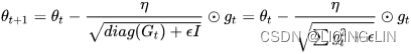
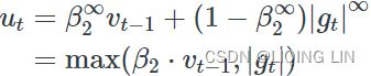
AdaGrad (adaptive gradient) : ###############
Consider the elongated bowl problem again: Gradient Descent starts by quickly going down the steepest slope, which does not point straight toward the global optimum, then it very slowly goes down to the bottom of the valley. It would be nice if the algorithm could correct its direction earlier to point a bit more toward the global optimum. The AdaGrad algorithm achieves this correction by scaling down the gradient vector along the steepest dimensions (see Equation 11-6).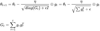
OR  # accumulates s 约束项regularizer: 1/

###########
# ![]() to denote the gradient at time step
to denote the gradient at time step 
# ![]() is then the partial derivative of the objective function w.r.t. to the parameter
is then the partial derivative of the objective function w.r.t. to the parameter  at time step :
 ![]()
# the general learning rate η at each time step for every parameter based on the past gradients that have been computed for: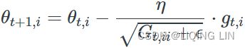
![]() is a diagonal matrix where each diagonal element
is a diagonal matrix where each diagonal element ![]() is the sum of the squares of the gradients w.r.t. up to time step
is the sum of the squares of the gradients w.r.t. up to time step
# As ![]() contains the sum of the squares of the past gradients w.r.t. to all parameters
contains the sum of the squares of the past gradients w.r.t. to all parameters  along its diagonal, we can now vectorize our implementation by performing a matrix-vector product⊙between
 ![]() and
and ![]() :
:
###########
Adagrad is an algorithm for gradient-based optimization that does just this: It adapts the learning rate to the parameters, performing smaller updates (i.e. low learning rates) for parameters associated with frequently occurring features(bigger (accumulates the square of the gradients) ==>
==>![]() is scaled down by a factor of ), and larger updates (i.e. high learning rates) for parameters associated with infrequent features(lower ). For this reason, it is well-suited for dealing with sparse data. Dean et al. have found that Adagrad greatly improved the robustness of SGD and used it for training large-scale neural nets at Google, which -- among other things -- learned to recognize cats in Youtube videos.
is scaled down by a factor of ), and larger updates (i.e. high learning rates) for parameters associated with infrequent features(lower ). For this reason, it is well-suited for dealing with sparse data. Dean et al. have found that Adagrad greatly improved the robustness of SGD and used it for training large-scale neural nets at Google, which -- among other things -- learned to recognize cats in Youtube videos.
特点:
it eliminates the need to manually tune the learning rate![]() ( It helps point the resulting updates more directly toward the global optimum). Most implementations use a default value of 0.01 and leave it at that.
( It helps point the resulting updates more directly toward the global optimum). Most implementations use a default value of 0.01 and leave it at that.
前期accumulates较小的时候,regularizer较大,能够放大梯度
后期accumulates较大的时候,regularizer较小,能够约束梯度
适合处理稀疏梯度
缺点:
由公式可以看出,仍依赖于人工设置一个全局学习率
learning rate设置过大的话,会使regularizer过于敏感,对梯度的调节太大
中后期,分母上梯度平方的累加将会越来越大,使 -->0,使gradent-->0,使得训练提前结束
Adagrad's main weakness is its accumulation of the squared gradients in the denominator: Since every added term is positive, the accumulated sum  keeps growing during training. This in turn causes the learning rate
![]() to shrink and eventually become infinitesimally small, at which point the algorithm is no longer able to acquire additional knowledge.
to shrink and eventually become infinitesimally small, at which point the algorithm is no longer able to acquire additional knowledge.
The first step accumulates the square of the gradients into the vector s (recall that the ⊗ symbol represents the element-wise multiplication ). This vectorized form is equivalent to computing for each element
  of the vector s; in other words, each accumulates the squares of the partial derivative of the cost function with regard to parameter . If the cost function is steep along the
  dimension, then
 will get larger and larger at each iteration.
The second step is almost identical to Gradient Descent, but with one big difference: the gradient vector is scaled down by a factor of s + ε (the ⊘ symbol represents the element-wise division, and ε is a smoothing term to avoid division by zero, typically set to  ). This vectorized form is equivalent to simultaneously computing
 for all parameters .
In short, this algorithm decays the learning rate, but it does so faster for steep陡峭 dimensions than for dimensions with gentler slopes平缓坡度. This is called an adaptive learning rate. It helps point the resulting updates more directly toward the global optimum (see Figure 11-7). One additional benefit is that it requires much less tuning of the learning rate hyperparameter η.
Figure 11-7. AdaGrad versus Gradient Descent: the former can correct its direction earlier to point to the optimum
AdaGrad frequently performs well for simple quadratic problems, but it often stops too early when training neural networks. The learning rate gets scaled down so much that the algorithm ends up stopping entirely before reaching the global optimum. So even though Keras has an Adagrad optimizer, you should not use it to train deep neural networks (it may be efficient for simpler tasks such as Linear Regression, though). Still, understanding AdaGrad is helpful to grasp the other adaptive learning rate optimizers.
OR # accumulates s 约束项regularizer: 1/

class AdaptiveGradientDescent(MiniBatchGradientDescent):
def __init__(self, epsilon=1e-6, **kwargs):
self.epsilon = epsilon
super(AdaptiveGradientDescent, self).__init__(**kwargs)
def fit(self, X, y):
X = np.c_[np.ones(len(X)), X]
n_samples, n_features = X.shape
self.theta = np.ones(n_features)
self.loss_ = [0]
gradient_sum = np.zeros(n_features)##############s
self.i = 0
while self.i < self.n_iter:
self.i += 1
if self.shuffle:
X, y = self._shuffle(X, y)
errors = []
for j in range(0, n_samples, self.batch_size):
mini_X, mini_y = X[j: j + self.batch_size], y[j: j + self.batch_size]
error = mini_X.dot(self.theta) - mini_y
errors.append(error.dot(error))
mini_gradient = 1 / self.batch_size * mini_X.T.dot(error)
gradient_sum += mini_gradient ** 2 ##############
adj_gradient = mini_gradient / (np.sqrt(gradient_sum + self.epsilon))
self.theta -= self.eta * adj_gradient
loss = 1 / (2 * self.batch_size) * np.mean(errors)
delta_loss = loss - self.loss_[-1]
self.loss_.append(loss)
if np.abs(delta_loss) < self.tolerance:
break
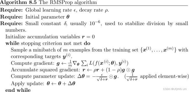
return selfRMSprop (Root Mean Square propagation) : ###############
As we’ve seen, AdaGrad runs the risk of slowing down a bit too fast and never converging to the global optimum. The RMSProp algorithm fixes this by accumulating only the gradients from the most recent iterations (as opposed to all the gradients since the beginning of training). It does so by using exponential decay in the first step (see Equation 11-7).
OR RMSprop as well divides the learning rate![]() by an exponentially decaying average of squared gradients.
by an exponentially decaying average of squared gradients.
Equation 11-7. RMSProp algorithm OR
OR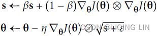
The decay rate β (or  )is typically set to 0.9. Yes, it is once again a new hyperparameter, but this default value often works well, so you may not need to tune it at all. while a good default value for the learning rate η is 0.001.
###########AdaGrad
# ![]() to denote the gradient at time step
to denote the gradient at time step
# ![]() is then the partial derivative of the objective function w.r.t. to the parameter at time step :
is then the partial derivative of the objective function w.r.t. to the parameter at time step : ![]()
# the general learning rate η at each time step for every parameter based on the past gradients that have been computed for:
![]() is a diagonal matrix where each diagonal element
is a diagonal matrix where each diagonal element ![]() is the sum of the squares of the gradients w.r.t. up to time step
is the sum of the squares of the gradients w.r.t. up to time step
# As ![]() contains the sum of the squares of the past gradients w.r.t. to all parameters along its diagonal, we can now vectorize our implementation by performing a matrix-vector product⊙between
contains the sum of the squares of the past gradients w.r.t. to all parameters along its diagonal, we can now vectorize our implementation by performing a matrix-vector product⊙between ![]() and
and ![]() :
:
########### OR
OR
class RMSProp(MiniBatchGradientDescent):
    def __init__(self, gamma=0.9, epsilon=1e-6, **kwargs):
        self.gamma = gamma #called momenturm B
        self.epsilon = epsilon
        super(RMSProp, self).__init__(**kwargs)

    def fit(self, X, y):
        X = np.c_[np.ones(len(X)), X]
        n_samples, n_features = X.shape
        self.theta = np.ones(n_features)
        self.loss_ = [0]

        gradient_exp = np.zeros(n_features)

        self.i = 0
        while self.i < self.n_iter:
            self.i += 1
            if self.shuffle:
                X, y = self._shuffle(X, y)

            errors = []
            for j in range(0, n_samples, self.batch_size):
                mini_X, mini_y = X[j: j + self.batch_size], y[j: j + self.batch_size]
                error = mini_X.dot(self.theta) - mini_y
                errors.append(error.dot(error))
                mini_gradient = 1 / self.batch_size * mini_X.T.dot(error)
                ###################################################
                gradient_exp = self.gamma * gradient_exp + (1 - self.gamma) * mini_gradient**2
                gradient_rms = np.sqrt(gradient_exp + self.epsilon)
                self.theta -= self.eta / gradient_rms * mini_gradient

            loss = 1 / (2 * self.batch_size) * np.mean(errors)
            delta_loss = loss - self.loss_[-1]
            self.loss_.append(loss)
            if np.abs(delta_loss) < self.tolerance:
                break
        return self
in tensor:tensorflow/rmsprop.py at master · tensorflow/tensorflow · GitHub
"""One-line documentation for rmsprop module.
rmsprop algorithm [tieleman2012rmsprop]
A detailed description of rmsprop.
- maintain a moving (discounted) average of the square of gradients
- divide gradient by the root of this average

mean_square = decay * mean_square{t-1} + (1-decay) * gradient ** 2
# momentum Defaults to 0.0.
mom = momentum * mom{t-1} + learning_rate * g_t /
        sqrt(mean_square + epsilon)
delta = - mom

This implementation of RMSProp uses plain momentum, not Nesterov momentum.
The centered version additionally maintains a moving (discounted) average of the
gradients, and uses that average to estimate the variance:

################
mean_grad = decay * mean_grad{t-1} + (1-decay) * gradient
################

mean_square = decay * mean_square{t-1} + (1-decay) * gradient ** 2
mom = momentum * mom{t-1} + learning_rate * g_t /
        sqrt(mean_square - mean_grad**2 + epsilon)
                           ############
delta = - mom
"""
in kera:keras/rmsprop.py at v2.10.0 · keras-team/keras · GitHub
centered : Boolean. If True, gradients are normalized by the estimated variance of the gradient通过梯度的估计方差对梯度进行归一化;
if False, by the uncentered second moment.OR
Setting this to True may help with training, but is slightly more expensive in terms of computation and memory. Defaults to False.
            ######224
            # mean_square: at iteration t, the mean of ( all gradients in mini-batch )
            # mean_square = decay * mean_square{t-1} + (1-decay) * gradient ** 2
            rms_t = coefficients["rho"] * rms
                    + coefficients["one_minus_rho"] * tf.square(grad)
            # tf.compat.v1.assign( ref, value, v
                                   alidate_shape=None, use_locking=None, name=None )
            # return : A Tensor that will hold the new value of ref
            #            after the assignment has completed
            # rms : is a tensor
            rms_t = tf.compat.v1.assign(
                rms, rms_t, use_locking=self._use_locking
            )# rms_t variable is refer to rms which was filled with new value
            denom_t = rms_t

            if self.centered:
                mg = self.get_slot(var, "mg")
                # mean: the mean of gradients from t=1 to t>1
                # -minus mean_grad at iteration t
                # mean_grad = decay * mean_grad{t-1} + (1-decay) * gradient
                mg_t = (
                    coefficients["rho"] * mg
                     + coefficients["one_minus_rho"] * grad
                )
                mg_t = tf.compat.v1.assign(
                    mg, mg_t, use_locking=self._use_locking
                )
                #######   mean_square + epsilon - mean_grad**2
                denom_t = rms_t - tf.square(mg_t)
            ######
            # momentum: Defaults to 0.0.
            # mom = momentum * mom{t-1} +
            #                    learning_rate * g_t / sqrt(mean_square + epsilon)
            # delta = - mom
            var_t = var - coefficients["lr_t"] * grad / (
                tf.sqrt(denom_t) + coefficients["epsilon"]
            )
            return tf.compat.v1.assign(
                var, var_t, use_locking=self._use_locking
            ).op
Adam (adaptive moment estimation) :###############
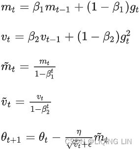
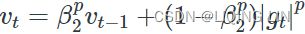
Adam, which stands for adaptive moment estimation自适应矩估计, combines the ideas of momentum optimization and RMSProp: just like momentum optimization, it keeps track of an exponentially decaying average of past gradients; and just like RMSProp, it keeps track of an exponentially decaying average of past squared gradients (see Equation 11-8).
Equation 11-8. Adam algorithm
1.  OR
OR
2. 
![]()
The only difference is that step 1 computes an exponentially decaying average rather than an exponentially decaying sum, but these are actually equivalent except for a constant factor (the decaying average is just ![]() times the decaying sum,
times the decaying sum, ![]() and
and ![]() are estimates of the first moment一阶矩 (the mean) of the gradient
are estimates of the first moment一阶矩 (the mean) of the gradient ![]() and the second moment二阶矩 (the uncentered variance) of the squared gradient
and the second moment二阶矩 (the uncentered variance) of the squared gradient ![]() at time step .
at time step .
As ![]() and
and ![]() are initialized as vectors of 0's, the authors of Adam observe that they are biased towards zero, especially during the initial time steps, and especially when the decay rates are small (i.e.
are initialized as vectors of 0's, the authors of Adam observe that they are biased towards zero, especially during the initial time steps, and especially when the decay rates are small (i.e.  and
and ![]() are close to 1)).
are close to 1)).
The momentum decay hyperparameter  is typically initialized to 0.9, while the scaling decay hyperparameter
  is often initialized to 0.999
3.  OR
OR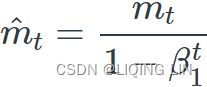 compute a bias correction
 ![]()
4. OR
OR 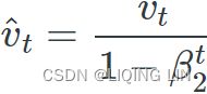 compute a bias correction
Steps 3 and 4 are somewhat of a technical detail: since  and are initialized at 0, they will be biased toward 0 at the beginning of training, so these two steps will help boost and at the beginning of training.
5.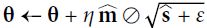 (
(![]() )OR
)OR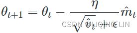 (unsigned
 ![]() )
)
If you just look at steps 1, 2, and 5, you will notice Adam’s close similarity to both momentum optimization and RMSProp. As earlier, the smoothing term ε is usually initialized to a tiny number such as  . These are the default values for the Adam class (to be precise, epsilon defaults to None, which tells Keras to use keras.backend.epsilon(), which defaults to ; you can change it using keras.backend.set_epsilon()).
Since Adam is an adaptive learning rate algorithm (like AdaGrad and RMSProp), it requires less tuning of the learning rate hyperparameter η. You can often use the default value η = 0.001, making Adam even easier to use than Gradient Descent.
可以看出,直接对梯度的矩估计对内存没有额外的要求,而且可以根据梯度进行动态调整,而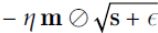 对学习率形成一个动态约束,而且有明确的范围。
特点:
结合了Adagrad善于处理稀疏梯度和RMSprop善于处理非平稳目标的优点
对内存需求较小
为不同的参数计算不同的自适应学习率
也适用于大多非凸优化- 适用于大数据集和高维空间
Note : in keras 偏差修正in learning rate:
# https://github.com/keras-team/keras/blob/b80dd12da9c0bc3f569eca3455e77762cf2ee8ef/keras/optimizers/optimizer_v2/adam.py
# 133
    def _prepare_local(self, var_device, var_dtype, apply_state):
        super()._prepare_local(var_device, var_dtype, apply_state)

        local_step = tf.cast(self.iterations + 1, var_dtype)
        beta_1_t = tf.identity(self._get_hyper("beta_1", var_dtype))
        beta_2_t = tf.identity(self._get_hyper("beta_2", var_dtype))
        beta_1_power = tf.pow(beta_1_t, local_step)
        beta_2_power = tf.pow(beta_2_t, local_step)
        # Correction
        lr = apply_state[(var_device, var_dtype)]["lr_t"] * (
            tf.sqrt(1 - beta_2_power) / (1 - beta_1_power)
        )
        apply_state[(var_device, var_dtype)].update(
            dict(
                lr=lr,
                epsilon=tf.convert_to_tensor(self.epsilon, var_dtype),
                beta_1_t=beta_1_t,
                beta_1_power=beta_1_power,
                one_minus_beta_1_t=1 - beta_1_t,
                beta_2_t=beta_2_t,
                beta_2_power=beta_2_power,
                one_minus_beta_2_t=1 - beta_2_t,
            )
        )
Adam相对于RMSProp新增了两处改动。其一,Adam使用经过指数移动加权 平均的梯度值(in mini-batch)来替换原始的梯度值;其二,Adam对经指数加权后的梯度值 ![]() 和平方梯度值
和平方梯度值 ![]() 都进行了修正,亦即偏差修正(Bias Correctionand)
都进行了修正,亦即偏差修正(Bias Correctionand)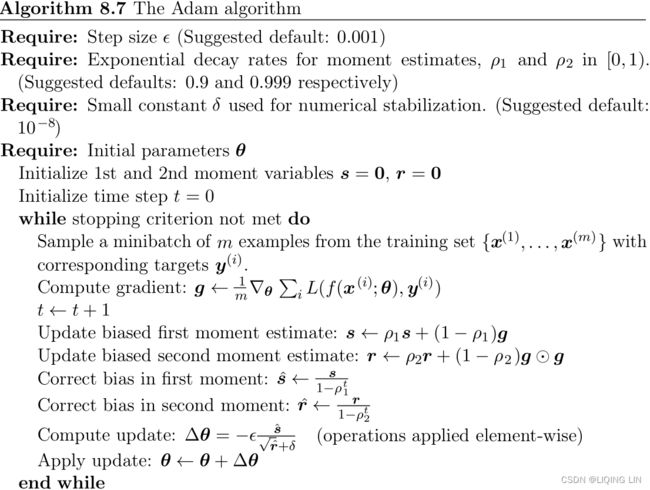
class AdaptiveMomentEstimation(MiniBatchGradientDescent):
    def __init__(self, beta_1=0.9, beta_2=0.999, epsilon=1e-6, **kwargs):
        self.beta_1 = beta_1
        self.beta_2 = beta_2
        self.epsilon = epsilon
        super(AdaptiveMomentEstimation, self).__init__(**kwargs)

    def fit(self, X, y):
        X = np.c_[np.ones(len(X)), X]
        n_samples, n_features = X.shape
        self.theta = np.ones(n_features)
        self.loss_ = [0]

        m_t = np.zeros(n_features)
        v_t = np.zeros(n_features)

        self.i = 0
        while self.i < self.n_iter:
            self.i += 1
            if self.shuffle:
                X, y = self._shuffle(X, y)
            errors = []
            for j in range(0, n_samples, self.batch_size):
                mini_X, mini_y = X[j: j + self.batch_size], y[j: j + self.batch_size]
                error = mini_X.dot(self.theta) - mini_y
                errors.append(error.dot(error))
                mini_gradient = 1 / self.batch_size * mini_X.T.dot(error)

                m_t = self.beta_1 * m_t + (1 - self.beta_1) * mini_gradient
                v_t = self.beta_2 * v_t + (1 - self.beta_2) * mini_gradient ** 2
                m_t_hat = m_t / (1 - self.beta_1 ** self.i)  # correction
                v_t_hat = v_t / (1 - self.beta_2 ** self.i)
                self.theta -= self.eta / (np.sqrt(v_t_hat) + self.epsilon) * m_t_hat

            loss = 1 / (2 * self.batch_size) * np.mean(errors)
            delta_loss = loss - self.loss_[-1]
            self.loss_.append(loss)
            if np.abs(delta_loss) < self.tolerance:
                break
        return self
AdaMax : ###############
1. OR
2. 
The ![]() factor in the Adam update rule scales the gradient inversely proportionally to the ℓ2 norm of the past gradients (via the
factor in the Adam update rule scales the gradient inversely proportionally to the ℓ2 norm of the past gradients (via the ![]() term) and current gradient
term) and current gradient ![]() :
:
Adam 2. ![]()
We can generalize this update to the ℓ![]() norm. Note that Kingma and Ba also parameterize
norm. Note that Kingma and Ba also parameterize ![]() as
as ![]() :
:
Norms for large ![]() values generally become numerically unstable, which is why ℓ
values generally become numerically unstable, which is why ℓ![]() and ℓ
and ℓ![]() norms are most common in practice. However, ℓ
norms are most common in practice. However, ℓ![]() also generally exhibits stable behavior. For this reason, the authors propose AdaMax (Kingma and Ba, 2015) and show that
also generally exhibits stable behavior. For this reason, the authors propose AdaMax (Kingma and Ba, 2015) and show that ![]() with ℓ
with ℓ![]() converges to the following more stable value. To avoid confusion with Adam, we use
converges to the following more stable value. To avoid confusion with Adam, we use  to denote the infinity norm-constrained
  :
:
3. OR compute a bias correction
We can now plug this into the Adam update equation by replacing ![]() with
with ![]() to obtain the AdaMax update rule:
to obtain the AdaMax update rule:
4. 
Note that as relies on the max operation, it is not as suggestible to bias towards zero偏向零并不容易 as  and in Adam, which is why we do not need to compute a bias correction for . Good default values are again η=0.002, β1=0.9, and β2=0.999.
class AdaMax(AdaptiveMomentEstimation):
    def __init__(self, **kwargs):
        super(AdaMax, self).__init__(**kwargs)

    def fit(self, X, y):
        X = np.c_[np.ones(len(X)), X]
        n_samples, n_features = X.shape
        self.theta = np.ones(n_features)
        self.loss_ = [0]

        m_t = np.zeros(n_features)
        u_t = np.zeros(n_features)
        beta_1=0.9, beta_2=0.999 #typically initialized

        self.i = 0
        while self.i < self.n_iter:
            self.i += 1
            if self.shuffle:
                X, y = self._shuffle(X, y)
            errors = []
            for j in range(0, n_samples, self.batch_size):
                mini_X, mini_y = X[j: j + self.batch_size], y[j: j + self.batch_size]
                error = mini_X.dot(self.theta) - mini_y
                errors.append(error.dot(error))
                mini_gradient = 1 / self.batch_size * mini_X.T.dot(error)

                m_t = self.beta_1 * m_t + (1 - self.beta_1) * mini_gradient
                m_t_hat = m_t / (1 - self.beta_1 ** self.i)###power
                u_t = np.max(np.c_[self.beta_2 * u_t, np.abs(mini_gradient)], axis=1)
                self.theta -= self.eta / u_t * m_t_hat
            loss = 1 / (2 * self.batch_size) * np.mean(errors)
            delta_loss = loss - self.loss_[-1]
            self.loss_.append(loss)
            if np.abs(delta_loss) < self.tolerance:
                break
return selfNadam:###############
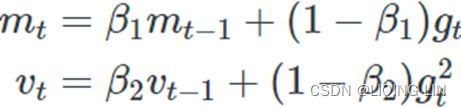
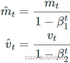
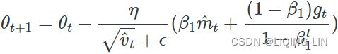
As we have seen before, Adam can be viewed as a combination of RMSpropand momentum
 : RMSprop contributes the exponentially decaying average of past squared gradients
 ![]() , while momentum accounts for the exponentially decaying average of past gradients . We have also seen that Nesterov accelerated gradient (NAG)
, while momentum accounts for the exponentially decaying average of past gradients . We have also seen that Nesterov accelerated gradient (NAG) is superior to vanilla momentum.
Nadam (Nesterov-accelerated Adaptive Moment Estimation) thus combines Adam and NAG. In order to incorporate NAG into Adam, we need to modify its momentum term .
First, let us recall the momentum update rule using our current notation :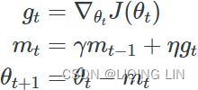 <==
<==
where  is our objective function,
  is the momentum decay term, and η is our step size(learning rate). Expanding the third equation above yields:
![]()
This demonstrates again that momentum involves taking a step in the direction of the previous momentum vector ![]() and a step in the direction of the current gradient
and a step in the direction of the current gradient  .
.
NAG then allows us to perform a more accurate step in the gradient direction by updating the parameters with the momentum step
![]() before computing the gradient
before computing the gradient![]() . We thus only need to modify the gradient to arrive at NAG:
. We thus only need to modify the gradient to arrive at NAG: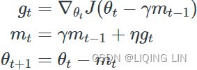 <==
<==
Dozat proposes to modify NAG the following way: Rather than applying the momentum step twice -- one time for updating the gradient and a second time for updating the parameters ![]() -- we now apply the look-ahead momentum vector directly to update the current parameters
-- we now apply the look-ahead momentum vector directly to update the current parameters![]() :
: 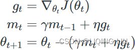
Notice that rather than utilizing the previous momentum vector ![]() as in the equation of the expanded momentum update rule above, we now use the current momentum vector to look ahead.
as in the equation of the expanded momentum update rule above, we now use the current momentum vector to look ahead.
In order to add Nesterov momentum to Adam, we can thus similarly replace the previous momentum vector![]() with the current momentum vector. First, recall that the Adam update rule is the following (note that we do not need to modify ):
with the current momentum vector. First, recall that the Adam update rule is the following (note that we do not need to modify ):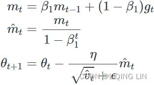 and
and ![]()
Expanding the 3rd equation with the definitions of ![]() and in turn gives us:
and in turn gives us: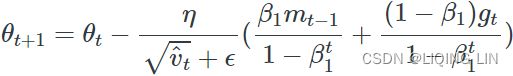
Note that ![]() is just the bias-corrected estimate of the momentum vector of the previous time step. We can thus replace it with
is just the bias-corrected estimate of the momentum vector of the previous time step. We can thus replace it with ![]() :
: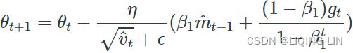
Note that for simplicity, we ignore that the denominator is ![]() and not
and not ![]() as we will replace the denominator in the next step anyway. This equation again looks very similar to our expanded momentum update rule above. We can now add Nesterov momentum just as we did previously
as we will replace the denominator in the next step anyway. This equation again looks very similar to our expanded momentum update rule above. We can now add Nesterov momentum just as we did previously![]() ==>
==>![]() by simply replacing this bias-corrected estimate of the momentum vector of the previous time step
by simply replacing this bias-corrected estimate of the momentum vector of the previous time step ![]() with the bias-corrected estimate of the current momentum vector
with the bias-corrected estimate of the current momentum vector ![]() , which gives us the Nadam update rule:
, which gives us the Nadam update rule:
可以看出,Nadam对学习率有了更强的约束,同时对梯度的更新也有更直接的影响。一般而言,在想使用带动量的RMSprop,或者Adam的地方,大多可以使用Nadam取得更好的效果。
Nadam optimization is Adam optimization plus the Nesterov trick, so it will often converge slightly faster than Adam. In his report introducing this technique, the researcher Timothy Dozat compares many different optimizers on various tasks and finds that Nadam generally outperforms Adam but is sometimes outperformed by RMSProp.
class Nadam(AdaptiveMomentEstimation):
    def __init__(self, **kwargs):
        super(Nadam, self).__init__(**kwargs)

    def fit(self, X, y):
        X = np.c_[np.ones(len(X)), X]
        n_samples, n_features = X.shape
        self.theta = np.ones(n_features)
        self.loss_ = [0]

        m_t = np.zeros(n_features)
        v_t = np.zeros(n_features)
        beta_1=0.9, beta_2=0.999 #typically initialized
        #beta_1 should be a list

        self.i = 0
        while self.i < self.n_iter:
            self.i += 1
            if self.shuffle:
                X, y = self._shuffle(X, y)
            errors = []
            for j in range(0, n_samples, self.batch_size):
                mini_X, mini_y = X[j: j + self.batch_size], y[j: j + self.batch_size]
                error = mini_X.dot(self.theta) - mini_y
                errors.append(error.dot(error))
                mini_gradient = 1 / self.batch_size * mini_X.T.dot(error)

                m_t = self.beta_1 * m_t + (1 - self.beta_1) * mini_gradient
                m_t_hat = m_t / (1 - self.beta_1 ** self.i)  # correction
                # since self.beta_1**self.i should be the multiplication of current beta_1 list

                v_t = self.beta_2 * v_t + (1 - self.beta_2) * mini_gradient ** 2
                v_t_hat = v_t / (1 - self.beta_2 ** self.i)

                self.theta -= self.eta / ( np.sqrt(v_t_hat) + self.epsilon ) *\
                              ( self.beta_1 * m_t_hat +\
                                (1 - self.beta_1) * mini_gradient /\
                                                 (1 - self.beta_1 ** self.i)
                              )

            loss = 1 / (2 * self.batch_size) * np.mean(errors)
            delta_loss = loss - self.loss_[-1]
            self.loss_.append(loss)
            if np.abs(delta_loss) < self.tolerance:
                break
        return self
Adaptive optimization methods (including RMSProp, Adam, and Nadam optimization) are often great, converging fast to a good solution. However, a 2017 paper###Ashia C. Wilson et al., “The Marginal Value of Adaptive Gradient Methods in Machine Learning,” Advances in Neural Information Processing Systems 30 (2017): 4148–4158.### by Ashia C. Wilson et al. showed that they can lead to solutions that generalize poorly on some datasets. So when you are disappointed by your model’s performance, try using plain Nesterov Accelerated Gradient instead: your dataset may just be allergic to adaptive gradients. Also check out the latest research, because it’s moving fast.
经验之谈
对于稀疏数据,尽量使用学习率可自适应的优化方法,不用手动调节,而且最好采用默认值
SGD通常训练时间更长,但是在好的初始化和学习率调度方案的情况下,结果更可靠
如果在意更快的收敛,并且需要训练较深较复杂的网络时,推荐使用学习率自适应adaptive learning rate的优化方法。
Adadelta,RMSprop,Adam是比较相近的算法,在相似的情况下表现差不多。
在想使用带动量的RMSprop,或者Adam的地方,大多可以使用Nadam取得更好的效果
Adadelta:###############
![]()
![\large \bigtriangleup \theta_t = - \frac{ \sqrt{E[\bigtriangleup \theta^2]_{t-1} + \epsilon} }{ \sqrt{ E[\bigtriangleup g^2]_{t} + \epsilon} } g_t](http://img.e-com-net.com/image/info8/34f2a52f576a48a4accd458d4920f4dc.gif)
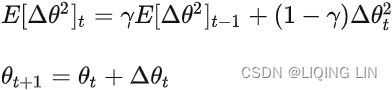
其中, 表示衰减参数。
Adadelta is an extension of Adagrad that seeks to reduce its aggressive, monotonically decreasing learning rate单调递减的学习率. Instead of accumulating all past squared gradients, Adadelta restricts the window of accumulated past gradients to some fixed size  .
.
Instead of inefficiently storing previous squared gradients, the sum of gradients is recursively defined as a decaying average of all past squared gradients. The running average ![]() at time step then depends (as a fraction similarly to the Momentum term) only on the previous average and the current gradient:
at time step then depends (as a fraction similarly to the Momentum term) only on the previous average and the current gradient:![]()
![]() : at iteration t, the mean of all gradients that are from all samples in mini-batch
: at iteration t, the mean of all gradients that are from all samples in mini-batch
We set to a similar value as the momentum term, around 0.9. For clarity, we now rewrite our vanilla SGD update in terms of the parameter update vector ![]() :
: <==SGD:
The parameter update vector of Adagrad that we derived previously thus takes the form: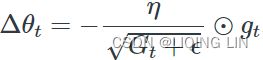
We now simply replace the diagonal matrix ![]() with the decaying average over past squared gradients
with the decaying average over past squared gradients ![]() :
: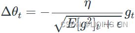
As the denominator is just the root mean squared (RMS) error criterion of the gradient, we can replace it with the criterion short-hand简写: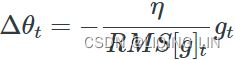
The authors note that the units in this update (as well as in SGD, Momentum, or Adagrad) do not match, i.e. the update should have the same hypothetical units as the parameter. To realize this, they first define another exponentially decaying average, this time not of squared gradients but of squared parameter updates:![]()
The root mean squared error of parameter updates is thus: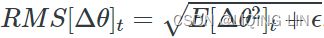
Since ![]() is unknown, we approximate it with the RMS of parameter updates until the previous time step
is unknown, we approximate it with the RMS of parameter updates until the previous time step ![]() . Replacing the learning rate
. Replacing the learning rate ![]() in the previous update rulewith
in the previous update rulewith ![]() finally yields the Adadelta update rule:
finally yields the Adadelta update rule: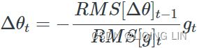 OR
OR![]()
With Adadelta, we do not even need to set a default learning rate, as it has been eliminated from the update rule.![]() 其中, γ 表示衰减参数。
其中, γ 表示衰减参数。
AdaDelta主要的特性在于其虽然考虑了历史的梯度值,但其通过对历史梯度的平方进行指数 加权 移动平均 来减缓梯度的累积效应![]() ,进而达到了减缓学习率收缩的速度;同时,其引入了一个作用类似于动量的成分
,进而达到了减缓学习率收缩的速度;同时,其引入了一个作用类似于动量的成分![]() and
and ![]() at
at ![]() 来代替原始的超参数学习率 η ,状态变量的自适应性加快了收敛速度
来代替原始的超参数学习率 η ,状态变量的自适应性加快了收敛速度
class AdaDelta(MiniBatchGradientDescent):
    def __init__(self, gamma=0.95, epsilon=1e-6, **kwargs):
        self.gamma = gamma
        self.epsilon = epsilon
        super(AdaDelta, self).__init__(**kwargs)

    def fit(self, X, y):
        X = np.c_[np.ones(len(X)), X]
        n_samples, n_features = X.shape
        self.theta = np.ones(n_features)
        self.loss_ = [0]

        gradient_exp = np.zeros(n_features)
        delta_theta_exp = np.zeros(n_features)

        self.i = 0
        while self.i < self.n_iter:
            self.i += 1
            if self.shuffle:
                X, y = self._shuffle(X, y)

            errors = []
            for j in range(0, n_samples, self.batch_size):
                mini_X, mini_y = X[j: j + self.batch_size], y[j: j + self.batch_size]
                error = mini_X.dot(self.theta) - mini_y
                errors.append(error.dot(error))
                mini_gradient = 1 / self.batch_size * mini_X.T.dot(error)

                gradient_exp = self.gamma * gradient_exp +\
                               (1 - self.gamma) * mini_gradient ** 2

                gradient_rms = np.sqrt( gradient_exp + self.epsilon )
                delta_theta = -np.sqrt( delta_theta_exp + self.epsilon ) /\
                              gradient_rms * mini_gradient

                delta_theta_exp = self.gamma * delta_theta_exp +\
                                  (1 - self.gamma) * delta_theta ** 2

                # delta_theta_rms = np.sqrt(delta_theta_exp + self.epsilon)
                # delta_theta = -delta_theta_rms / gradient_rms * mini_gradient

                self.theta += delta_theta

            loss = 1 / (2 * self.batch_size) * np.mean(errors)
            delta_loss = loss - self.loss_[-1]
            self.loss_.append(loss)
            if np.abs(delta_loss) < self.tolerance:
                break
        return self
in keras:https://github.com/keras-team/keras/blob/b80dd12da9c0bc3f569eca3455e77762cf2ee8ef/keras/optimizers/optimizer_v2/adadelta_test.py
                        # 102
                        # Perform initial update without previous accum values
                        accum = accum * rho + (grad**2) * (1 - rho)
                        update[step] = ( np.sqrt( accum_update + epsilon )
                                         * ( 1.0 / np.sqrt(accum + epsilon) )
                                         * grad
                                       )
                        accum_update = accum_update * rho +\
                                       ( update[step] ** 2 ) * (1.0 - rho)
                        tot_update += update[step] * lr
AMSGrad : ###############
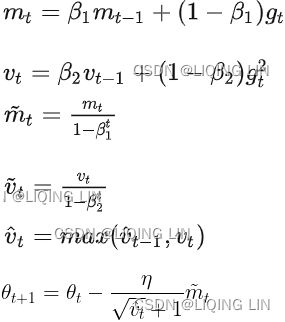
As adaptive learning rate methods have become the norm in training neural networks, practitioners noticed that in some cases, e.g. for object recognition or machine translation they fail to converge to an optimal solution and are outperformed by SGD with momentum在动量方面优于 SGD.
Reddi et al. (2018) formalize this issue and pinpoint the exponential moving average of past squared gradients as a reason for the poor generalization behaviour of adaptive learning rate methods. Recall that the introduction of the exponential average was well-motivated: It should prevent the learning rates to become infinitesimally small as training progresses, the key flaw of the Adagrad algorithm. However, this short-term memory of the gradients becomes an obstacle in other scenarios.
In settings where Adam converges to a suboptimal solution, it has been observed that some minibatches provide large and informative gradients, but as these minibatches only occur rarely, exponential averaging diminishes their influence, which leads to poor convergence. The authors provide an example for a simple convex optimization problem(https://blog.csdn.net/Linli522362242/article/details/104124771Gradient Descent cannot get stuck in a local minimum when training a Logistic Regression model because the cost function is convex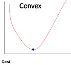 ) where the same behaviour can be observed for Adam.
To fix this behaviour, the authors propose a new algorithm, AMSGrad that uses the maximum of past squared gradients ![]() rather than the exponential average to update the parameters.
rather than the exponential average to update the parameters. ![]() is defined the same as in Adam above:
is defined the same as in Adam above:![]()
Instead of using ![]() (or its bias-corrected version
(or its bias-corrected version ![]() , in keras' learning rate) directly, we now employ the previous
, in keras' learning rate) directly, we now employ the previous ![]() if it is larger than the current one:
if it is larger than the current one:![]()
This way, AMSGrad results in a non-increasing step size, which avoids the problems suffered by Adam.
For simplicity, the authors also remove the debiasing step that we have seen in Adam. The full AMSGrad update without bias-corrected estimates can be seen below: 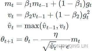
class AMSGrad(AdaptiveMomentEstimation):
    def __init__(self, **kwargs):
        super(AMSGrad, self).__init__(**kwargs)

    def fit(self, X, y):
        X = np.c_[np.ones(len(X)), X]
        n_samples, n_features = X.shape
        self.theta = np.ones(n_features)
        self.loss_ = [0]

        m_t = np.zeros(n_features)
        v_t = np.zeros(n_features)
        v_t_hat = np.zeros(n_features)

        self.i = 0
        while self.i < self.n_iter:
            self.i += 1
            if self.shuffle:
                X, y = self._shuffle(X, y)
            errors = []
            for j in range(0, n_samples, self.batch_size):
                mini_X, mini_y = X[j: j + self.batch_size], y[j: j + self.batch_size]
                error = mini_X.dot(self.theta) - mini_y
                errors.append(error.dot(error))
                mini_gradient = 1 / self.batch_size * mini_X.T.dot(error)

                m_t = self.beta_1 * m_t + (1 - self.beta_1) * mini_gradient
                v_t = self.beta_2 * v_t + (1 - self.beta_2) * mini_gradient ** 2
                v_t_hat = np.max(
                                    np.hstack( (v_t_hat, v_t) )
                                ) # concatenation along the second axis
                self.theta -= self.eta / (np.sqrt(v_t_hat) + self.epsilon) * m_t

            loss = 1 / (2 * self.batch_size) * np.mean(errors)
            delta_loss = loss - self.loss_[-1]
            self.loss_.append(loss)
            if np.abs(delta_loss) < self.tolerance:
                break
        return self
Note: keras uses the debiasing steps(bias-corrected version) that we have seen in Adam

![]()
![]()
# adam.py
# https://github.com/keras-team/keras/blob/b80dd12da9c0bc3f569eca3455e77762cf2ee8ef/keras/optimizers/optimizer_v2/adam.py
# 133
def _prepare_local(self, var_device, var_dtype, apply_state):
super()._prepare_local(var_device, var_dtype, apply_state)
local_step = tf.cast(self.iterations + 1, var_dtype)
beta_1_t = tf.identity(self._get_hyper("beta_1", var_dtype))
beta_2_t = tf.identity(self._get_hyper("beta_2", var_dtype))
beta_1_power = tf.pow(beta_1_t, local_step)
beta_2_power = tf.pow(beta_2_t, local_step)
# Correction
lr = apply_state[(var_device, var_dtype)]["lr_t"] * (
tf.sqrt(1 - beta_2_power) / (1 - beta_1_power)
)
apply_state[(var_device, var_dtype)].update(
dict(
lr=lr,
epsilon=tf.convert_to_tensor(self.epsilon, var_dtype),
beta_1_t=beta_1_t,
beta_1_power=beta_1_power,
one_minus_beta_1_t=1 - beta_1_t,
beta_2_t=beta_2_t,
beta_2_power=beta_2_power,
one_minus_beta_2_t=1 - beta_2_t,
)
)
# OR adam_test.py
# https://github.com/keras-team/keras/blob/v2.10.0/keras/optimizers/optimizer_v2/adam_test.py
# 39
def adam_update_numpy_amsgrad(
param, g_t, t, m, v, vhat, lr=0.001, beta1=0.9, beta2=0.999, epsilon=1e-7
):
# Correction
lr_t = lr * np.sqrt(1 - beta2 ** (t + 1)) / (1 - beta1 ** (t + 1))
m_t = beta1 * m + (1 - beta1) * g_t
v_t = beta2 * v + (1 - beta2) * g_t * g_t
vhat_t = np.maximum(vhat, v_t)
param_t = param - lr_t * m_t / (np.sqrt(vhat_t) + epsilon)
return param_t, m_t, v_t, vhat_tNewton's method
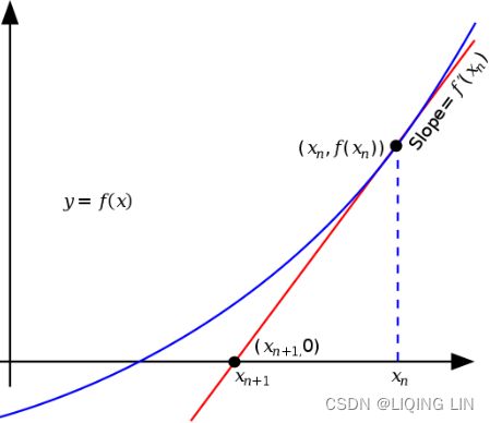
 https://blog.csdn.net/Linli522362242/article/details/125662545
Use the function  to find the roots of the equation
  (i.e. all solutions to x that give . For example:
 ![]() , then x=2 and x=3 are both the roots of function .
, then x=2 and x=3 are both the roots of function .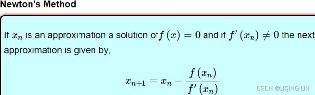
A graphical representation of Newton's method is shown in the following screenshot.  is the initial x value. The derivative of
  is evaluated, which is a tangent line crossing the x axis at
  . The iteration is repeated, evaluating the derivative at points ,
  and so on:
 ==>
==>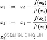 ==>
==>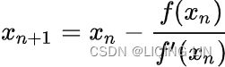
Newton's method, also known as the Newton-Raphson method, uses an iterative procedure to solve for a root using information about the derivative of a function. The derivative is treated as a linear problem to be solved. The first-order derivation, , of the function,, represents the tangent line. The approximation to the next value of , given as , is as follows:
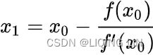 ==>
==>![]()
 ==>
==>![]()
Here, the tangent line intersects the x axis at , which produces y=0. This also represents the first-order Taylor expansion about , such that that the new pont, ![]() , solves the following equation:
, solves the following equation: ![]()
This process is repeated with x taking the value of  until the maximum number of iterations is reached, or the absolute difference between
  and is within an acceptable accuracy level.
An initial guess value is required to compute需要一个初始猜测值来计算 the values of and . The rate of convergence is quadratic收敛速度是二次的, which is considered to be extremely fast at obtaining the solution with high levels of accuracy.
The drawback to Newton's method is that it does not guarantee global convergence to the solution. Such a situation arises when the function contains more than one root, or when the algorithm arrives at a local extremum and is unable to compute the next step. As this method requires knowledge of the derivative of its input function, it is required that the input function be differentiable. However, in certain circumstances, it is impossible for the derivative of a function to be known, or otherwise be mathematically easy to compute.
The implementation of Newton's method in Python is as follows:
# The Newton-Raphson method

def newton(func, df, x, tol=0.001, maxiter=100):
    """
    :param func: The function to solve
    :param df: The derivative function of f
    :param x: Initial guess value of x
    :param tol: The precision of the solution
    :param maxiter: Maximum number of iterations
    :return:
        The x-axis value of the root,
        number of iterations used
    """
    n = 1
    while n<=maxiter:
        x1 = x-func(x)/df(x)
        if abs(x1-x) < tol: # the Root is very close
            return x1, n
        x = x1
        n += 1
return None, n![]() ==>
==> ![]() : the input function be differentiable
: the input function be differentiable
# The keyword 'lambda' creates an anonymous function
# with input argument x
# https://blog.csdn.net/Linli522362242/article/details/107086444
# return x**3 + 2.*x**2 - 5
y = lambda x: x**3 + 2.*x**2 - 5
dy = lambda x: 3.*x**2 + 4.*x
# x start from 5
root, iterations = newton( y, dy, 5., 0.00001, 100 )
print( "Root is:", root )
print( "Iterations:", iterations )
print( "y:", root**3 + 2.*root**2 - 5)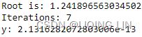 Beware of division by zero exceptions! In Python 2, using values such as 5.0, instead of 5, lets Python recognize the variable as a float, avoids the problem of treating variables as integers in calculations, and gives us better precision.
With Newton's method, we obtained a really close solution with less iteration over the bisection method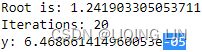
2 利用牛顿法求驻点(Stationary point, 也即求解函数的解)
1. find the roots of the equation (i.e. all solutions to x that give
==>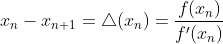
to find such that 
OR 

so let ![]() when
when ![]() ,
,![]()
OR ![]() and
and ![]()
2.当函数 的一阶导数为 时,点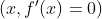 为函数的驻点。############
求某函数![]() 的驻点(A stationary point, or critical point, is a point at which the curve's gradient equals to zero.
的驻点(A stationary point, or critical point, is a point at which the curve's gradient equals to zero. ![]() ,即为求解该函数的导函数的根( (i.e. all solutions to x that give
,即为求解该函数的导函数的根( (i.e. all solutions to x that give ![]() ),故同样可以利用牛顿法求解。
),故同样可以利用牛顿法求解。
Suppose: 
then we use Newton's method to find the root of  or (i.e. all solutions to x that give
 ![]() or
or ![]()
if exists  such that
 ![]()
then ![]()
and ![]()
then 
OR![]()
If the multiplicity m of the root is finite then ![]() will have a root at the same location with multiplicity 1. Applying Newton's method to find the root of g(x) recovers quadratic convergence in many cases although it generally involves the second derivative of f(x). In a particularly simple case, if
will have a root at the same location with multiplicity 1. Applying Newton's method to find the root of g(x) recovers quadratic convergence in many cases although it generally involves the second derivative of f(x). In a particularly simple case, if ![]() ( is differentiable, so we can get
( is differentiable, so we can get ![]() ) then
) then![]() ==>
==> ![]() ==>
==>![]() and Newton's method finds the root of g(x) in a single iteration with
and Newton's method finds the root of g(x) in a single iteration with 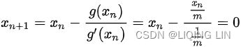
for example: ![]()
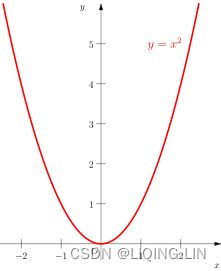 ==>
==>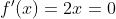 ==>the root of (here
 ![]() ==>
==> ![]() such that
such that ![]() , so
, so ![]() 为函数的驻点)
为函数的驻点)
let ![]() ==>
==> ![]()
via an iteration with Newton's method to find such that ![]()
when ![]() and
and ![]()
![]()
OR![]()
so the point( ![]() ) is the point which is the closest to stationary point(
) is the point which is the closest to stationary point( ![]() )
)
3. from Newton's method to Taylor polynomial
is infinitely differentiable,
![]()
![]()
![]()
==> ![]()
![]()
Assume ![]() :
:![]()
![]()
![]()
Assume ![]()
then![]()
![]()
Assume ![]()
![]()
![]()
![]()
...
If only the point is considered near the extreme point , that is to say, all ![]() are the same value and are near the extreme point :
are the same value and are near the extreme point : ![]()
![]()
this is Taylor polynomial.
4. From Taylor polynomial to Newton’s method ######################
牛顿法法主要是为了解决非线性优化问题,其收敛速度比梯度下降速度更快。其需要解决的问题可以描述为:对于目标函数,在无约束条件的情况下求它的最小值。
Newton’s method is a second-order method in the simplest setting where we consider unconstrained smooth convex optimization (same as the setting for gradient descent).![]() OR
OR ![]()
其中x= 是n维空间的向量。我们在下面需要用到的泰勒公式先在这写出来。
OR![]()
牛顿法的主要思想是:在现有的极小值![]() 附近的估计值
附近的估计值 (或者只考虑 在极值点
 ![]() 附近)对做二阶泰勒展开,进而找到极小点的下一个估计值
附近)对做二阶泰勒展开,进而找到极小点的下一个估计值 (或者
(或者![]() ),反复迭代直到函数的一阶导数小于某个接近0的阀值。
),反复迭代直到函数的一阶导数小于某个接近0的阀值。
- 给多长的增量
 ,能使得点
,能使得点  为极值点
为极值点 (或者近似的极值点),换言之希望此时
  ≈0。
≈0。
与梯度下降一样,取前3项, OR 对函数 进行泰勒展开到2阶:
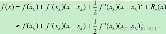
令两边相等,等式两边同时对![]() 求导, 其导数
求导, 其导数![]() and
and ![]() ,
,![]() 即:
即:![]()
![]()
OR![]() ==>
==>
由于![]() ,所以参数更新公式为:
,所以参数更新公式为:![]() ==>
==>![]()
由此,我们可以得出结论:牛顿法的本质是泰勒级数的二阶展开
5. 多元函数的求导问题 #############################################
https://zhuanlan.zhihu.com/p/218676280
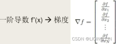
![]() ==>
==>![]() or
or ![]()
![]()
![]()
Example:
Equation 4-1. Linear Regression model prediction (X0==1, X0 *  ==, the bias term also is w0 ):
cost function:OR
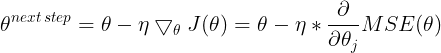
![]() is learning rate or step size
is learning rate or step size
if ![]() , and
, and ![]() , then
, then ![]() ,
, 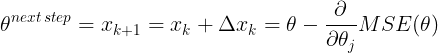
Equation 4-5. Partial derivatives of the cost function(start with  or sample index i >=1)
 j: feature index
Instead of computing these gradients individually, you can use Equation 4-6 to compute them all in one go. The gradient vector, noted  , contains all the partial derivatives of the cost function (one for each model parameter, or weight
 ![]() ).
).
Equation 4-6. Gradient vector of the cost function ( for equation 4-5)

https://blog.csdn.net/Linli522362242/article/details/104005906
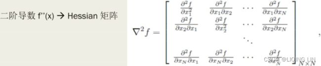 Example:
https://blog.csdn.net/Linli522362242/article/details/126672904
support vector classifier (SVC)
 Here, N is the number of samples in our dataset.
- Positive hyperplane :

- Negative hyperplane:

- ==>
 (constraint) and
sub-Summary: to solve (classs label
![]() )
)
==>At first,(to find the closest of data points to decision boundary(![]() OR
OR ![]() ),
),
Then maximize for maximizing the margin( to choose the decision boundary or to find the support vectors that determine the location boundary) ==> (maximize ==> is equivalent to minimizing )
==>
In order to solve this constrained optimization (maximize) problem, we introduce Lagrange multipliers拉格朗日乘数, with one multiplier for each of the constraints in (7.5==>
 ), giving the Lagrangian function
  ###we put the constraints together
where a =  . Note the minus sign in front of the Lagrange multiplier term, because we are minimizing with respect to w and b, and maximizing with respect to
  OR
OR for .==>convert to==>
Setting the derivatives of L(w, b, a) with respect to w and b equal to zero, we obtain the following two conditions
the partial derivatives of L (w, b, a)=0 ==> ==>
==>
the partial derivatives of L (w, b, a)=0 ==> ==>
==> 
Eliminating w and b from L(w, b, a) using these conditions
replaced with
 *
* 
and,  ==
== +
+
==> 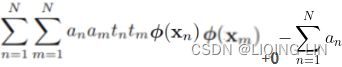
Then, minus
minus ==>
==>
 ==>
==>
then gives the dual representation of the maximum margin problem in which we maximize

with respect to a subject to the constraints
The hard margin(without slacks variables)
 a = the constraints
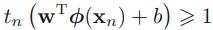


Quadratic Programming
https://blog.csdn.net/Linli522362242/article/details/104280075
Equation 5-5. Quadratic Programming problem #p is a vertical vector  OR
OR
 ==>
==> ==>
==>
 mpf2_线性规划_CAPM_sharpe_Arbitrage Pricin_Inversion Gauss Jordan_Statsmodel_Pulp_pLU_Cholesky_QR_Jacobi_LIQING LIN的博客-CSDN博客
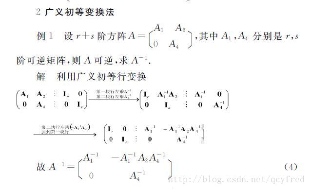
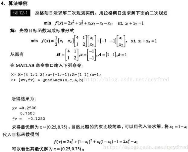
example: 
 ==>
==> ==>
==> code: https://blog.csdn.net/Linli522362242/article/details/104280075
H= ![]() , c=f=
, c=f=![]() , A=
, A= , b=
, b=
Newton’s Method
the first-order methods
Introduce step size![]() or
or ![]()
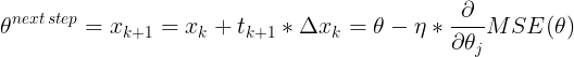
the second-order methods
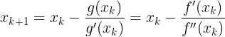
Duality plays a very fundamental role in designing second-order methods for convex optimization. Newton’s method is a second-order method in the simplest setting where we consider unconstrained smooth convex optimization (same as the setting for gradient descent).
![]()
Recall that in gradient descent, the update in the th iteration, ![]() moved in the direction of the negative gradient of the previous iteration(the first-order methods)
moved in the direction of the negative gradient of the previous iteration(the first-order methods)![]()
where ![]() is the step-size. In contrast, in Newton’s method we move in the direction of negative Hessian inverse of the gradient.
is the step-size. In contrast, in Newton’s method we move in the direction of negative Hessian inverse of the gradient.![]()
OR ![]()
This is called the pure Newton’s method, since there’s no notion of a step size![]() involved(the second-order methods). As is evident from the update, Newton’s method involves solving linear systems in the Hessian.
involved(the second-order methods). As is evident from the update, Newton’s method involves solving linear systems in the Hessian.
To motivate Newton’s method, consider the following quadratic approximation
(Suppose, we have an estimate  and we want our next estimate
 ![]() to have the property that
to have the property that ![]() )
)![]()
![]()
###############
The Newton update is obtained by minimizing the above w.r.t. ![]() . This quadratic approximation is better than the approximation used in gradient descent (given by 14.1), since it uses more information about the function via the Hessian.
. This quadratic approximation is better than the approximation used in gradient descent (given by 14.1), since it uses more information about the function via the Hessian.![]()
###############
In order to simplify much of the notation, we’re going to think of our iterative algorithm of producing a sequence of such quadratic approximations ![]() . Without loss of generality, we can write
. Without loss of generality, we can write ![]() and re-write the above equation,
and re-write the above equation,![]() where
where ![]() and
and ![]() represent the gradient and Hessian of at
represent the gradient and Hessian of at ![]() .
.
We want to choose Δx to minimize this local quadratic approximation of at ![]() . Differentiating with respect to Δx above yields:
. Differentiating with respect to Δx above yields:

Recall that any Δx which yields ![]() is a local extrema of
is a local extrema of ![]() (⋅). If we assume that
(⋅). If we assume that ![]() is [postive definite]
is [postive definite]
(psd:############

the identity matrix ![]() or
or  is positive-definite
正定矩阵ppt - 百度文库
特征值判别法 ==>
==>
即 matrix A is positive-definite
https://zh.m.wikipedia.org/wiki/%E6%AD%A3%E5%AE%9A%E7%9F%A9%E9%98%B5https://en.wikipedia.org/wiki/Definite_matrixhttps://zh.m.wikipedia.org/wiki/%E6%AD%A3%E5%AE%9A%E7%9F%A9%E9%98%B5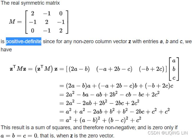 https://zh.m.wikipedia.org/wiki/%E6%AD%A3%E5%AE%9A%E7%9F%A9%E9%98%B5
############) then we know this Δx is also a global minimum for hn(⋅). Solving for Δx:![]() <==
<==![]() <==
<==
where ![]() and
and ![]() represent the gradient and Hessian of at
represent the gradient and Hessian of at ![]() , and
, and ![]() is the approximate Newton's direction
is the approximate Newton's direction
This suggests ![]() as a good direction to move
as a good direction to move ![]() towards. In practice, we set
towards. In practice, we set ![]() for a value of
for a value of  where
where ![]() is ‘sufficiently’ smaller than
is ‘sufficiently’ smaller than ![]() .
. 
The computation of the step-size(learning rate) can use any number of line search algorithms. The simplest of these is backtracking line search, where you simply try smaller and smaller values of until the function value is ‘small enough’.
In terms of software engineering, we can treat NewtonRaphson as a blackbox for any twice-differentiable function
Quasi-Newton
Suppose that instead of requiring ![]() be the inverse hessian at
be the inverse hessian at ![]() , we think of it as an approximation of this information. We can generalize NewtonRaphson to take a QuasiUpdate policy which is responsible for producing a sequence of
, we think of it as an approximation of this information. We can generalize NewtonRaphson to take a QuasiUpdate policy which is responsible for producing a sequence of ![]() .
.
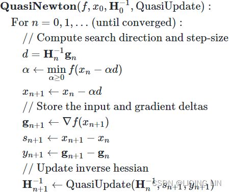 We’ve assumed that QuasiUpdate only requires the former inverse hessian estimate as well as the input and gradient differences (sn and yn respectively). Note that if QuasiUpdate just returns
 ![]() , we recover exact NewtonRaphson. In terms of software, we can blackbox optimize an arbitrary differentiable function (with no need to be able to compute a second derivative) using QuasiNewton assuming we get a quasi-newton approximation update policy.
, we recover exact NewtonRaphson. In terms of software, we can blackbox optimize an arbitrary differentiable function (with no need to be able to compute a second derivative) using QuasiNewton assuming we get a quasi-newton approximation update policy.
Note that the only use we have of the hessian is via it’s product with the gradient direction(less memory). This will become useful for the L-BFGS algorithm described below, since we don’t need to represent the Hessian approximation in memory. If you want to see these abstractions in action.
Behave like a Hessian
What form should QuasiUpdate take? Well, if we have QuasiUpdate always return the identity matrix (ignoring its inputs), then this corresponds to simple gradient descent, since the search direction is always ![]() . While this actually yields a valid procedure which will converge to for convex , intuitively this choice of QuasiUpdate isn’t attempting to capture second-order information about .
. While this actually yields a valid procedure which will converge to for convex , intuitively this choice of QuasiUpdate isn’t attempting to capture second-order information about .
Let’s think about our choice of  as an approximation for near
 ![]() : Note
: Note ![]() is a scalar
is a scalar vs
vs![]()
Secant Condition
A good property for ![]() is that its gradient
is that its gradient ![]() agrees with(和.. 一致) at
agrees with(和.. 一致) at ![]() and
and ![]() . In other words, we’d like to ensure:
. In other words, we’d like to ensure: 
Using both of the equations above: ![]()
Using the gradient of ![]() (⋅) and canceling terms we get
(⋅) and canceling terms we get ![]()
This yields the so-called “secant conditions” which ensures that ![]() behaves like the Hessian at least for the diference
behaves like the Hessian at least for the diference ![]() . Assuming
. Assuming ![]() is invertible (which is true if it is psd), then multiplying both sides by
is invertible (which is true if it is psd), then multiplying both sides by ![]() yields :
yields :![]() <==
<==![]()
where  is the difference in gradients and
  is the difference in inputs.
Recall that the a hessian represents the matrix of 2nd order partial derivatives: ![]() . The hessian is symmetric since the order of differentiation doesn’t matter.
. The hessian is symmetric since the order of differentiation doesn’t matter.
BFGS
The Broyden–Fletcher–Goldfarb–Shanno (BFGS) algorithm attempts to bring some of the advantages of Newton’s method without the computational burden. In that respect, BFGS is similar to CG. However, BFGS takes a more direct approach to the approximation of Newton’s update. Recall that Newton’s update is given by ![]()
![]()
![]() and α is the step-size
and α is the step-size
where H is the Hessian of with respect to θ evaluated at  . The primary computational difficulty in applying Newton’s update is the calculation of the inverse Hessian
  . The approach adopted by quasi-Newton methods (of which the BFGS algorithm is the most prominent) is to approximate the inverse with a matrix
  that is iteratively refined by low rank updates to become a better approximation of .
Once the inverse Hessian approximation is updated, the direction of descent ![]() is determined by
is determined by ![]() . A line search is performed in this direction to determine the size of the step,
. A line search is performed in this direction to determine the size of the step, ![]() , taken in this direction. The final update to the parameters is given by:
, taken in this direction. The final update to the parameters is given by:![]()

Like the method of conjugate gradients, the BFGS algorithm iterates a series of line searches with the direction incorporating second-order information. However unlike conjugate gradients(共轭梯度法(英語:Conjugate gradient method),是求解系数矩阵为对称正定矩阵的线性方程组的数值解的方法。共轭梯度法是一个迭代方法,它适用于系数矩阵为稀疏矩阵的线性方程组,因为使用像Cholesky分解 https://blog.csdn.net/Linli522362242/article/details/125546725这样的直接方法求解这些系统所需的计算量太大了。这种方程组在数值求解偏微分方程时很常见。 ==>
==>![]()
 ==>==>
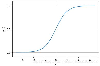
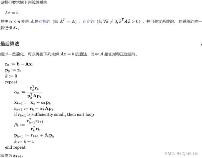 ), the success of the approach is not heavily dependent on the line search finding a point very close to the true minimum along the line. Thus, relative to conjugate gradients, BFGS has the advantage that it can spend less time refining each line search. On the other hand, the BFGS algorithm must store the inverse Hessian matrix, M , that requires
 ![]() memory, making BFGS impractical不切实际 for most modern deep learning models that typically have millions of parameters.
memory, making BFGS impractical不切实际 for most modern deep learning models that typically have millions of parameters.
The BFGS Update
Intuitively, we want ![]() to satisfy the two conditions:
to satisfy the two conditions:
- Secant condition holds for
 and
and 
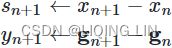
The curvature condition should be satisfied for
  to be positive definite, which can be verified by pre-multiplying the secant equation with
  .
. - is symmetric
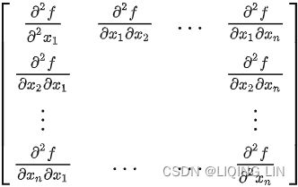
Given the two conditions above, we’d like to take the most conservative change relative to ![]() . This is reminiscent of the MIRA update, where we have conditions on any good solution but all other things equal, want the ‘smallest’ change.
. This is reminiscent of the MIRA update, where we have conditions on any good solution but all other things equal, want the ‘smallest’ change. 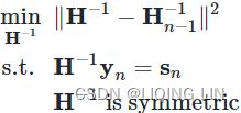
The norm used here ∥⋅∥ is the weighted frobenius norm. The solution to this optimization problem is given by![]()
where ![]() . Proving this is relatively involved and mostly symbol crunching.
. Proving this is relatively involved and mostly symbol crunching.
This update is known as the Broyden–Fletcher–Goldfarb–Shanno (BFGS) update, named after the original authors. Some things worth noting about this update
-
 is positive definite (psd) when
  is. Assuming our initial guess of
  is psd, it follows by induction each inverse Hessian estimate is as well. Since we can choose any
  we want, including the
  matrix, this is easy to ensure.
 -
The above also specifies a recurrence relationship between
and . We only need the history of and to re-construct .
The last point is significant since it will yield a procedural algorithm for computing ![]() , for a direction
, for a direction  , without ever forming the
 ![]() matrix. Repeatedly applying the recurrence above we have
matrix. Repeatedly applying the recurrence above we have
From an initial guess (or![]() )and an approximate inverted Hessian matrix
)and an approximate inverted Hessian matrix ![]() the following steps are repeated as converges to the solution:
the following steps are repeated as converges to the solution:
For k = 0, ... (until converged):
- 1. Obtain a direction
 (or
(or  ) by solving
  (or
(or 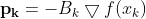 )
)
If is initialized with
  , the first step will be equivalent to a gradient descent, but further steps are more and more refined by
  , the approximation to the Hessian.
where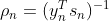
OR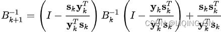
This can be computed efficiently without temporary matrices, recognizing that is symmetric, and that
  and
and  are scalars, using an expansion such as
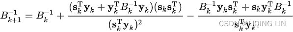
Therefore, in order to avoid any matrix inversion, must be the approximation of the inverse of the Hessian instead of the Hessian approximation: - 2. Perform a one-dimensional optimization (line search) to find an acceptable stepsize
 (OR
(OR  )in the direction found in the first step. If an exact line search is performed, then
  or(
or( ) . In practice, an inexact line search usually suffices不精确的线搜索通常就足够了, with an acceptable
  satisfying Wolfe conditions.
 - 3.set
 and update
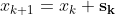
- 4.
 OR
OR 
- 5.

Since the only use for ![]() is via the product
is via the product ![]() , we only need the above procedure to use the BFGS approximation in QuasiNewton.
, we only need the above procedure to use the BFGS approximation in QuasiNewton.
OR
We also assume that we have stored the last m updates of the form(m=batch_size)
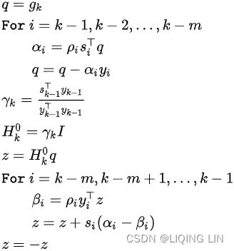
The BFGS quasi-newton approximation has the benefit of not requiring us to be able to analytically compute the Hessian of a function. However, we still must maintain a history of the and  vectors for each iteration. Since one of the core-concerns of the NewtonRaphson algorithm were the memory requirements associated with maintaining an Hessian, the BFGS Quasi-Newton algorithm doesn’t address that since our memory use can grow without bound.
Limited Memory BFGS (or L-BFGS)
The memory costs of the BFGS algorithm can be significantly decreased by avoiding storing the complete(nxm = the total number of training samples x the number of features ==> batch_size x the number of features) inverse Hessian approximation M OR![]() . The L-BFGS algorithm computes the approximation M using the same method as the BFGS algorithm, but beginning with the assumption that
. The L-BFGS algorithm computes the approximation M using the same method as the BFGS algorithm, but beginning with the assumption that ![]() is the identity matrix单位矩阵, rather than storing the approximation from one step to the next. If used with exact line searches, the directions defined by L-BFGS are mutually conjugate. However, unlike the method of conjugate gradients, this procedure remains well behaved when the minimum of the line search is reached only approximately. Th L-BFGS strategy with no storage described here can be generalized to include more information about the Hessian by storing some of the vectors used to update at each time step, which costs only per step.
is the identity matrix单位矩阵, rather than storing the approximation from one step to the next. If used with exact line searches, the directions defined by L-BFGS are mutually conjugate. However, unlike the method of conjugate gradients, this procedure remains well behaved when the minimum of the line search is reached only approximately. Th L-BFGS strategy with no storage described here can be generalized to include more information about the Hessian by storing some of the vectors used to update at each time step, which costs only per step.
The L-BFGS algorithm, named for limited BFGS, simply truncates the BFGSMultiply update to use the last m input differences and gradient differences. This means, we only need to store  and
and ![]() to compute the update. The center product can still use any symmetric psd matrix
to compute the update. The center product can still use any symmetric psd matrix ![]() , which can also depend on any {sk}{sk} or {yk}.
, which can also depend on any {sk}{sk} or {yk}.
Numerical Optimization: Understanding L-BFGS — aria42
https://en.wikipedia.org/wiki/Limited-memory_BFGS
https://en.wikipedia.org/wiki/Broyden%E2%80%93Fletcher%E2%80%93Goldfarb%E2%80%93Shanno_algorithm说说牛顿迭代 -- 方法篇 - 知乎
- Rprop (resilient backpropagation)
Adam is a popular choice of optimizer, and is seen as a combination of RMSprop and SGD with momentum. It is an adaptive learning rate optimization algorithm, computing individual learning rates for different parameters.
#################################
Learning Rate η Scheduling
To find a good learning rate, you can use grid search (see04_TrainingModels_03_LIQING LIN的博客-CSDN博客)
Finding a good learning rate is very important. If you set it much too high, training may diverge (as we discussed in “Gradient Descent” on page 118). If you set it too low, training will eventually converge to the optimum, but it will take a very long time. If you set it slightly too high, it will make progress very quickly at first, but it will end up dancing around the optimum, never really settling down. If you have a limited computing budget, you may have to interrupt training before it has converged properly, yielding a suboptimal solution (see Figure 11-8).
Figure 11-8. Learning curves for various learning rates η
As we discussed in Chapter 10 https://blog.csdn.net/Linli522362242/article/details/106849041 One way to find a good learning rate is to train the model for a few hundred iterations, starting with a very low learning rate (e.g.,  ) and gradually increasing it up to a very large value (e.g., 10). This is done by multiplying the learning rate by a constant factor at each iteration (e.g., by
 ![]() =0.03261938194, to 10 in 500 iterations). the optimal learning rate will be a bit lower than the turning point at which the loss starts to climb (typically about 10 times lower than the turning point), you can find a good learning rate by training the model for a few hundred iterations, exponentially increasing the learning rate from a very small value to a very large value, and then looking at the learning curve and picking a learning rate slightly lower than the one at which the learning curve starts shooting back up. You can then reinitialize your model and train it with that learning rate.
=0.03261938194, to 10 in 500 iterations). the optimal learning rate will be a bit lower than the turning point at which the loss starts to climb (typically about 10 times lower than the turning point), you can find a good learning rate by training the model for a few hundred iterations, exponentially increasing the learning rate from a very small value to a very large value, and then looking at the learning curve and picking a learning rate slightly lower than the one at which the learning curve starts shooting back up. You can then reinitialize your model and train it with that learning rate.
Note
In stochastic gradient descent implementations, the fixed learning rate ![]() is often replaced by an adaptive learning rate that decreases over time, for example,where and are constants. Note that stochastic gradient descent does not reach the global minimum but an area very close to it. By using an adaptive learning rate, we can achieve further annealing磨炼 to a better global minimum
is often replaced by an adaptive learning rate that decreases over time, for example,where and are constants. Note that stochastic gradient descent does not reach the global minimum but an area very close to it. By using an adaptive learning rate, we can achieve further annealing磨炼 to a better global minimum
theta_path_sgd = []
m=len(X_b)
np.random.seed(42)

n_epochs = 50
t0,t1= 5,50

def learning_schedule(t):
    return t0/(t+t1)

theta = np.random.randn(2,1)

for epoch in range(n_epochs): # n_epochs=50 replaces n_iterations=1000
    for i in range(m): # m = len(X_b)
        if epoch==0 and i<20:
            y_predict = X_new_b.dot(theta)
            style="b-" if i>0 else "r--"
            plt.plot(X_new,y_predict, style)######

        random_index = np.random.randint(m)  ##### Stochastic
        xi = X_b[random_index:random_index+1]
        yi = y[random_index:random_index+1]
        gradients = 2*xi.T.dot( xi.dot(theta) - yi ) ##### Gradient
        eta=learning_schedule(epoch*m + i) ############## e.g. 5/( (epoch*m+i)+50)
        theta = theta-eta * gradients  ###### Descent
        theta_path_sgd.append(theta)


plt.plot(X, y, "b.")
plt.xlabel("$x_1$", fontsize=18)
plt.ylabel("$y$", rotation=0, fontsize=18)
plt.title("Figure 4-10. Stochastic Gradient Descent first 10 steps")

plt.axis([0,2, 0,15])
plt.show()
https://blog.csdn.net/Linli522362242/article/details/104005906
But you can do better than a constant learning rate: if you start with a large learning rate and then reduce it once training stops making fast progress, you can reach a good solution faster than with the optimal constant learning rate. There are many different strategies to reduce the learning rate during training. It can also be beneficial to start with a low learning rate, increase it, then drop it again. These strategies are called learning schedule:
Power scheduling幂调度(&Time-based)
Set the learning rate to a function of the iteration step  (#I believe is iterations in keras#):
 ![]() . The initial learning rate
. The initial learning rate ![]() , the power
, the power  (typically set to 1
VS
Time-based learning schedules alter the learning rate depending on the learning rate of the previous time iteration. Factoring in the decay the mathematical formula for the learning rate is:
![]()
), and the steps  (#I believe is
 ![]() in keras OR
in keras OR  #) are hyperparameters. The learning rate drops at each step.
After t=1 iteration step and s=1, it is down to ![]() .
.
After t=2 iteration steps and s=1, it is down to ![]() ,
,
then it goes down to ![]() , then
, then ![]() , and so on. As you can see, this schedule first drops quickly, then more and more slowly. Of course, power scheduling requires tuning
, and so on. As you can see, this schedule first drops quickly, then more and more slowly. Of course, power scheduling requires tuning ![]() and (and possibly
and (and possibly  ).
).
# https://github.com/tensorflow/tensorflow/blob/v2.2.0/tensorflow/python/keras/optimizers.py
# 210-213
class SGD(Optimizer):
  """Stochastic gradient descent optimizer.
  Includes support for momentum,
  learning rate decay, and Nesterov momentum.
  Arguments:
      lr: float >= 0. Learning rate.
      momentum: float >= 0. Parameter that accelerates SGD in the relevant
        direction and dampens oscillations.
      decay: float >= 0. Learning rate decay over each update.
      nesterov: boolean. Whether to apply Nesterov momentum.
  """

  def __init__(self, lr=0.01, momentum=0., decay=0., nesterov=False, **kwargs):
    super(SGD, self).__init__(**kwargs)
    with K.name_scope(self.__class__.__name__):
      self.iterations = K.variable(0, dtype='int64', name='iterations')
      self.lr = K.variable(lr, name='lr')
      self.momentum = K.variable(momentum, name='momentum')
      self.decay = K.variable(decay, name='decay')
    self.initial_decay = decay
    self.nesterov = nesterov

  def _create_all_weights(self, params):
    shapes = [K.int_shape(p) for p in params]
    moments = [K.zeros(shape) for shape in shapes]
    self.weights = [self.iterations] + moments
    return moments

  def get_updates(self, loss, params):
    grads = self.get_gradients(loss, params)
    self.updates = [state_ops.assign_add(self.iterations, 1)]

    lr = self.lr
    if self.initial_decay > 0:
      lr = lr * (  # pylint: disable=g-no-augmented-assignment
          1. /
          (1. +
           self.decay * math_ops.cast(self.iterations, K.dtype(self.decay))))
Implementing power scheduling in Keras is the easiest option: just set the decay hyperparameter when creating an optimizer:
The decay ( ) is the inverse of (the number of steps it takes to divide the learning rate by one more unit, such as ![]() ), and Keras assumes that
), and Keras assumes that  .
. ![]() and is iterations
and is iterations
#class SGD(tensorflow.python.keras.optimizer_v2.optimizer_v2.OptimizerV2)
# |  SGD(learning_rate=0.01, momentum=0.0, nesterov=False, name='SGD', **kwargs)
optimizer = keras.optimizers.SGD( lr=0.01, decay=1e-4)


import tensorflow as tf
import numpy as np

tf.random.set_seed(42)
np.random.seed(42)

model = keras.models.Sequential([
    keras.layers.Flatten(input_shape=[28,28]), # 1D arrray: 28*28
    keras.layers.Dense( 300, activation="selu", kernel_initializer="lecun_normal" ),#Scaled ELU
    keras.layers.Dense( 100, activation="selu", kernel_initializer="lecun_normal" ),
    keras.layers.Dense( 10, activation="softmax")
])

model.compile(loss="sparse_categorical_crossentropy", optimizer=optimizer, metrics=["accuracy"])

n_epochs=25
history = model.fit( X_train_scaled, y_train, epochs=n_epochs,
                     validation_data=(X_valid_scaled, y_valid)
                   )
... ...
![]() and is iterations
and is iterations
we have a total of 55,000 training samples, and
model.fit(batch_size=None) ==> If unspecified, batch_size will default to 32.that implies there are a total of ![]() steps per epoch( n_steps_per_epoch = len(X_train) //batch_size ). Therefore, a total of n_steps_per_epoch weight updates need to be applied before an epoch completes.==>iterationSteps =
steps per epoch( n_steps_per_epoch = len(X_train) //batch_size ). Therefore, a total of n_steps_per_epoch weight updates need to be applied before an epoch completes.==>iterationSteps =![]() = n_steps_per_epoch * epoch_index
= n_steps_per_epoch * epoch_index
To see an example of the Time-based learning schedules calculation, our initial learning rate is ![]() and our
and our ![]() . (note, if decay=0, then we will use Constant Learning Rate
. (note, if decay=0, then we will use Constant Learning Rate ![]() )
)![]()
import matplotlib.pyplot as plt

learning_rate = 0.01
decay = 1e-4
batch_size=32
n_steps_per_epoch = len(X_train) //batch_size
epochs = np.arange(n_epochs)
                                 # = iteration step = 25 epochs * n_steps_per_epoch
lrs = learning_rate / (1 + decay * epochs*n_steps_per_epoch )

plt.plot( epochs, lrs, "o-")
plt.axis([0, n_epochs-1, 0, 0.01])
plt.xlabel("Epoch")
plt.ylabel("Learning Rate")
plt.title("Power Scheduling", fontsize=14)
plt.grid(True)
plt.show()
![]()
# https://github.com/keras-team/keras/blob/v2.10.0/keras/optimizers/schedules/learning_rate_schedule.py#L467-L572
# 548 - 572
    def __call__(self, step):
        with tf.name_scope(self.name or "InverseTimeDecay") as name:
            initial_learning_rate = tf.convert_to_tensor(
                self.initial_learning_rate, name="initial_learning_rate"
            )
            dtype = initial_learning_rate.dtype
            decay_steps = tf.cast(self.decay_steps, dtype)
            decay_rate = tf.cast(self.decay_rate, dtype)

            global_step_recomp = tf.cast(step, dtype)
            p = global_step_recomp / decay_steps
            if self.staircase:
                p = tf.floor(p)
            const = tf.cast(tf.constant(1), dtype)
            denom = tf.add(const, tf.multiply(decay_rate, p))
            return tf.divide(initial_learning_rate, denom, name=name)
# class SGD(tensorflow.python.keras.optimizer_v2.optimizer_v2.OptimizerV2)
# | SGD(learning_rate=0.01, momentum=0.0, nesterov=False, name='SGD', **kwargs)
# optimizer = keras.optimizers.SGD( lr=0.01, decay=1e-4)
initial_learning_rate = 0.01
decay = 1e-4
decay_steps = 1
learning_rate_fn = keras.optimizers.schedules.InverseTimeDecay( initial_learning_rate,
decay_steps,
decay )
# https://github.com/keras-team/keras/blob/v2.10.0/keras/optimizers/schedules/learning_rate_schedule.py#L467-L572
# 557-558
# global_step_recomp = tf.cast(step, dtype) #
# p = global_step_recomp / decay_steps
import tensorflow as tf
import numpy as np
tf.random.set_seed(42)
np.random.seed(42)
model = keras.models.Sequential([
keras.layers.Flatten(input_shape=[28,28]), # 1D arrray: 28*28
keras.layers.Dense( 300, activation="selu", kernel_initializer="lecun_normal" ),
keras.layers.Dense( 100, activation="selu", kernel_initializer="lecun_normal" ),
keras.layers.Dense( 10, activation="softmax")
])
model.compile(loss="sparse_categorical_crossentropy",
optimizer=keras.optimizers.SGD(learning_rate=learning_rate_fn),
metrics=["accuracy"])
n_epochs=25
history = model.fit( X_train_scaled, y_train, epochs=n_epochs, validation_data=(X_valid_scaled, y_valid) )Exponential Decay scheduling
Set the learning rate to ![]() OR
OR ![]() . The learning rate will gradually drop by a factor of 10 every
. The learning rate will gradually drop by a factor of 10 every  . While power scheduling reduces the learning rate more and more slowly, exponential scheduling keeps slashing大幅削减 it by a factor of 10 every
 ![]() .
.
# 98 - 194
@keras_export("keras.optimizers.schedules.ExponentialDecay")
class ExponentialDecay(LearningRateSchedule):
  """A LearningRateSchedule that uses an exponential decay schedule."""

  def __init__(
      self,
      initial_learning_rate,
      decay_steps,
      decay_rate,
      staircase=False,
      name=None):
    """Applies exponential decay to the learning rate.
    ```python
    def decayed_learning_rate(step):
      return initial_learning_rate * decay_rate ^ (step / decay_steps)
    ```
    ```python
    You can pass this schedule directly into a `tf.keras.optimizers.Optimizer`
    as the learning rate.
    Example: When fitting a Keras model, decay every 100000 steps with a base
    of 0.96:

    initial_learning_rate = 0.1
    lr_schedule = tf.keras.optimizers.schedules.ExponentialDecay(
        initial_learning_rate,
        decay_steps=100000,
        decay_rate=0.96,
        staircase=True)
    model.compile(optimizer=tf.keras.optimizers.SGD(learning_rate=lr_schedule),
                  loss='sparse_categorical_crossentropy',
                  metrics=['accuracy'])
    model.fit(data, labels, epochs=5)
    ```
    Args:
      initial_learning_rate: A scalar `float32` or `float64` `Tensor` or a
        Python number.  The initial learning rate.
      decay_steps: A scalar `int32` or `int64` `Tensor` or a Python number.
        Must be positive.  See the decay computation above.
      decay_rate: A scalar `float32` or `float64` `Tensor` or a
        Python number.  The decay rate.
      staircase: Boolean.  If `True` decay the learning rate at discrete
        intervals
      name: String.  Optional name of the operation.  Defaults to
        'ExponentialDecay'.
    """
    super(ExponentialDecay, self).__init__()
    self.initial_learning_rate = initial_learning_rate
    self.decay_steps = decay_steps
    self.decay_rate = decay_rate
    self.staircase = staircase
    self.name = name

  def __call__(self, step):
    with ops.name_scope_v2(self.name or "ExponentialDecay") as name:
      initial_learning_rate = ops.convert_to_tensor_v2(
          self.initial_learning_rate, name="initial_learning_rate")     # initial_learning_rate
      dtype = initial_learning_rate.dtype
      decay_steps = math_ops.cast(self.decay_steps, dtype)
      decay_rate = math_ops.cast(self.decay_rate, dtype)                # 0.1

      global_step_recomp = math_ops.cast(step, dtype)
      p = global_step_recomp / decay_steps                              # t/s=step /decay_steps
      if self.staircase:
        p = math_ops.floor(p)
      return math_ops.multiply(
          initial_learning_rate, math_ops.pow(decay_rate, p), name=name)#initial_learning_rate*decay_rate^(t/s)
update learning rate per epoch (epoch >=1)
Exponential scheduling and piecewise scheduling are quite simple too. You first need to define a function that takes the current epoch and returns the learning rate. For example, let’s implement exponential scheduling:![]()
def exponential_decay_fn(epoch):
    return 0.01 * 0.1**(epoch / 20)
If you do not want to hardcode ![]() and , you can create a function that returns a configured function:
and , you can create a function that returns a configured function:
# initial_learning_rate = 0.01
# lr_schedule = tf.keras.optimizers.schedules.ExponentialDecay(
#     initial_learning_rate,
#     decay_steps=20,
#     decay_rate=0.1,
#     staircase=True
# )

# You first need to define a function that takes the current epoch and returns the
# learning rate. For example, let’s implement exponential scheduling:
# def exponential_decay_fn(epoch): #per epoch or current iteration 't'
#     return 0.01 * 0.1**(epoch/20)

def exponential_decay(lr0, s): # def exponential_decay(lr0=0.01, s=20):
    def exponential_decay_fn(epoch): #epoch is global_step_recomp or step or 't'
        return lr0 * 0.1**(epoch/s)
    return exponential_decay_fn #不加括号就是返回函数对象,不是函数调用


exponential_decay_fn = exponential_decay(lr0=0.01, s=20)

model = keras.models.Sequential([
    keras.layers.Flatten( input_shape=[28,28]),
    keras.layers.Dense(300, activation="selu", kernel_initializer="lecun_normal"),
    keras.layers.Dense(100, activation="selu", kernel_initializer="lecun_normal"),
    keras.layers.Dense(10, activation="softmax")
])

model.compile( loss="sparse_categorical_crossentropy", optimizer="nadam", metrics=["accuracy"])
n_epochs = 25
Next, create a LearningRateScheduler callback, giving it the schedule function, and pass this callback to the fit() method:
lr_scheduler = keras.callbacks.LearningRateScheduler( exponential_decay_fn )
history = model.fit(X_train_scaled, y_train, epochs=n_epochs,
                    validation_data=(X_valid_scaled, y_valid),
                    callbacks=[lr_scheduler])
The LearningRateScheduler will update the optimizer’s learning_rate attribute at the beginning of each epoch. Updating the learning rate once per epoch is usually enough, but if you want it to be updated more often, for example at every step, you can always write your own callback (see the “Exponential Scheduling” section of the notebook for an example). Updating the learning rate at every step makes sense if there are many steps per epoch. Alternatively, you can use the keras.optimizers.schedules approach, described shortly.
find_learning_rate
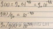 ==>
==>
==>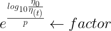 ==>
==>![\LARGE \eta_0 * [ e^{ \frac{log_{10}\frac{\eta_0}{\eta_{(t)}}} {p}}]^n = \eta_0[factor]^n](http://img.e-com-net.com/image/info8/0979b72da535442c9468d1aba35f1b74.gif)
K = keras.backend

class ExponentialLearningRate(keras.callbacks.Callback):
    def __init__(self, factor):
        self.factor = factor
        self.rates = []
        self.losses = []
    def on_batch_end(self, batch, logs):
        self.rates.append( K.get_value(self.model.optimizer.learning_rate) )
        self.losses.append( logs["loss"] )
        K.set_value( self.model.optimizer.learning_rate,
                     self.model.optimizer.learning_rate * self.factor
                   )

def find_learning_rate( model, X, y, epochs=1, batch_size=32,
                        min_rate=10**-5, max_rate=10
                      ):
    init_weights = model.get_weights()

    iterations = math.ceil( len(X) / batch_size ) * epochs
    factor = np.exp( np.log(max_rate / min_rate) / iterations )

    init_lr = K.get_value(model.optimizer.learning_rate)

    K.set_value( model.optimizer.learning_rate, min_rate )
    exp_lr = ExponentialLearningRate( factor )
    history = model.fit( X, y, epochs=epochs, batch_size=batch_size,
                         callbacks=[exp_lr]
                       )

    K.set_value( model.optimizer.learning_rate, init_lr )
    model.set_weights(init_weights)

    return exp_lr.rates, exp_lr.losses

def plot_lr_vs_loss( rates, losses ):
    plt.plot(rates, losses)
    plt.gca().set_xscale("log")
    plt.hlines( min(losses), min(rates),max(rates) )
    plt.axis( [min(rates), max(rates),  min(losses), (losses[0]+min(losses))/2 ])
    plt.xlabel("Learning rate")
plt.ylabel("Loss") Warning: In the
 on_batch_end() method, logs["loss"] used to contain the batch loss, but in TensorFlow 2.2.0 it was replaced with the mean loss (since the start of the epoch). This explains why the graph below is much smoother than in the book (if you are using TF 2.2 or above). It also means that there is a lag between the moment the batch loss starts exploding and the moment the explosion becomes clear in the graph. So you should choose a slightly smaller learning rate than you would have chosen with the "noisy" graph. Alternatively, you can tweak the ExponentialLearningRate callback above so it computes the batch loss (based on the current mean loss and the previous mean loss):
class ExponentialLearningRate(keras.callbacks.Callback):
    def __init__(self, factor):
        self.factor = factor
        self.rates = []
        self.losses = []

    def on_epoch_begin(self, epoch, logs=None):
        self.prev_loss = 0

    def on_batch_end(self, batch, logs=None):
        batch_loss = logs["loss"] * (batch + 1) - self.prev_loss * batch

        self.prev_loss = logs["loss"]

        # self.rates.append( K.get_value(self.model.optimizer.lr) )
        self.rates.append( K.get_value(self.model.optimizer.learning_rate) )
        self.losses.append( batch_loss )
        K.set_value( self.model.optimizer.learning_rate,
                     self.model.optimizer.learning_rate * self.factor
                   )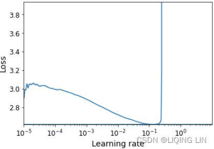
update learning rate per epoch (epoch >=0)
The schedule function can take the current learning rate as a second argument: For example, the following schedule function multiplies the previous learning rate by , which results in the same exponential decay (except the decay now starts at the beginning of epoch 0 instead of 1):
def exponential_decay_fn(epoch, current_lr):
    return current_lr*0.1**(1/20) #    decay_steps=20, decay_rate=0.1, steps=t=current epoch when ignoring epoch value
Updating the learning rate once 20 epoch: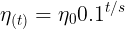
t : global_step_recomp = tf.cast(step, dtype)
# s : decay steps
s = 20 * len(X_train) // 32 # number of steps in '20 epochs' (batch size = 32)
learning_rate = keras.optimizers.schedules.ExponentialDecay(0.01, s, 0.1)
optimizer = keras.optimizers.SGD(learning_rate)
When you save a model, the optimizer and its learning rate get saved along with it. This means that with this new schedule function, you could just load a trained model and continue training where it left off, no problem. Things are not so simple if your schedule function uses the epoch argument, however: the epoch does not get saved![]() , and it gets reset to 0 every time you call the fit() method. If you were to continue training a model where it left off, this could lead to a very large learning rate, which would likely damage your model’s weights. One solution is to manually set the fit() method’s initial_epoch argument so the epoch starts at the right value.(the
, and it gets reset to 0 every time you call the fit() method. If you were to continue training a model where it left off, this could lead to a very large learning rate, which would likely damage your model’s weights. One solution is to manually set the fit() method’s initial_epoch argument so the epoch starts at the right value.(the initial_epoch argument let you specify the initial value(=4) of current epoch to start from when training)
#Training first 4 Epcohs and saving
model.fit(x_train, y_train, validation_data=(x_val, y_val), batch_size=32, epochs=4)
model.save("partial.h5")


#loading the model, training another 4 Epochs and then saving the updated model.
from keras.models import load_model
new_model = load_model('partial.h5')
new_model.fit(x_train, y_train, validation_data=(x_val, y_val), batch_size=32,
              initial_epoch=4,
              epochs=25)
new_model.save("updated.h5")
update the learning rate per batch
If you want to update the learning rate at each iteration (each batch) rather than at each epoch (n_epochs=25), you must write your own callback class:
K = keras.backend

class ExponentialDecay( keras.callbacks.Callback ):
    def __init__(self, s=40000): #s: decay_steps
        super().__init__()
        self.s = s

    def on_batch_begin(self, batch, logs=None):
    # def on_epoch_begin(self, epoch, logs=None):
        ### Original
        ### batch: integer, index of batch within the current epoch. #each epoch has batch_size=32
        ### the learing rate is updated at each poch
        #now
        #  the learing rate is updated at each batch
        # Note: the `batch` argument is reset at each epoch
        lr = K.get_value(self.model.optimizer.lr)
        #print('\nbatch: ', batch, ' learing rate: ', lr,'\n')
        K.set_value(self.model.optimizer.lr, lr*0.1**(1/s)) #s: decay_steps #s = 20*len(X_train)//32

    def on_epoch_end( self, epoch, logs=None):
        logs = logs or {}
        logs['lr'] = K.get_value(self.model.optimizer.lr)

model = keras.models.Sequential([
    keras.layers.Flatten(input_shape=[28,28]),
    keras.layers.Dense(300, activation="selu", kernel_initializer="lecun_normal"),
    keras.layers.Dense(100, activation="selu", kernel_initializer="lecun_normal"),
    keras.layers.Dense(10, activation="softmax")
])

lr0=0.01
optimizer = keras.optimizers.Nadam(lr=lr0)
model.compile( loss="sparse_categorical_crossentropy", optimizer=optimizer, metrics=['accuracy'])
n_epochs=25

s = 20*len(X_train)//32  # number of steps in 20 epochs (batch size = 32)
exp_decay = ExponentialDecay(s)
history = model.fit(X_train_scaled, y_train, epochs=n_epochs,
                    validation_data = (X_valid_scaled, y_valid),
                    callbacks=[exp_decay])
Piecewise constant scheduling分段恒定调度:
Use a constant learning rate for a number of epochs (e.g., ![]() for 5 epochs), then a smaller learning rate for another number of epochs (e.g.,
for 5 epochs), then a smaller learning rate for another number of epochs (e.g.,  for 50 epochs), and so on. Although this solution can work very well, it requires fiddling around to figure out the right sequence of learning rates and how long to use each of them.
#https://github.com/keras-team/keras/blob/v2.10.0/keras/optimizers/schedules/learning_rate_schedule.py#L206-L311
# 206-
@keras_export("keras.optimizers.schedules.PiecewiseConstantDecay")
class PiecewiseConstantDecay(LearningRateSchedule):
    """A LearningRateSchedule that uses a piecewise constant decay schedule.
    The function returns a 1-arg callable to compute the piecewise constant
    when passed the current optimizer step. This can be useful for changing the
    learning rate value across different invocations of optimizer functions.
    Example: use a learning rate that's
            1.0 for the first 100000 steps,
            0.5 for the next   10000 steps, and
            0.1 for any additional steps.
    ```python
    step = tf.Variable(0, trainable=False)
    boundaries = [100000, 110000]
    values = [1.0,
              0.5,
              0.1]
    learning_rate_fn = keras.optimizers.schedules.PiecewiseConstantDecay(
                                                    boundaries, values
                                                  )
    # Later, whenever we perform an optimization step, we pass in the step.
    learning_rate = learning_rate_fn(step)
    ```
    You can pass this schedule directly into a `tf.keras.optimizers.Optimizer`
    as the learning rate. The learning rate schedule is also serializable and
    deserializable using `tf.keras.optimizers.schedules.serialize` and
    `tf.keras.optimizers.schedules.deserialize`.
    Returns:
      A 1-arg callable learning rate schedule that takes the current optimizer
      step and outputs the decayed learning rate, a scalar `Tensor` of the same
      type as the boundary tensors.

      The output of the 1-arg function that takes
      the `step` is
         `values[0]` when `step <= boundaries[0]`,
         `values[1]` when `step > boundaries[0]` and `step <= boundaries[1]`, ...,
      and values[-1] when `step > boundaries[-1]`.
    """

    def __init__(self, boundaries, values, name=None):
        """Piecewise constant from boundaries and interval values.
        Args:
          boundaries: A list of `Tensor`s or `int`s or `float`s with strictly
            increasing entries, and with all elements having the same type as
            the optimizer step.
          values: A list of `Tensor`s or `float`s or `int`s that specifies the
            values for the intervals defined by `boundaries`. It should have one
            more element than `boundaries`, and all elements should have the
            same type.
          name: A string. Optional name of the operation. Defaults to
            'PiecewiseConstant'.
        Raises:
          ValueError: if the number of elements in the lists do not match.
        """
        super().__init__()

        if len(boundaries) != len(values) - 1:
            raise ValueError(
                "The length of boundaries should be 1 less than the length of "
                f"values. Received: boundaries={boundaries} of length "
                f"{len(boundaries)}, and values={values} "
                f"of length {len(values)}."
            )

        self.boundaries = boundaries
        self.values = values
        self.name = name

    def __call__(self, step):
        with tf.name_scope(self.name or "PiecewiseConstant"):
            boundaries = tf.nest.map_structure(
                tf.convert_to_tensor, tf.nest.flatten(self.boundaries)
            )
            values = tf.nest.map_structure(
                tf.convert_to_tensor, tf.nest.flatten(self.values)
            )
            x_recomp = tf.convert_to_tensor(step)

            for i, b in enumerate(boundaries):
                if b.dtype.base_dtype != x_recomp.dtype.base_dtype:
                    # We cast the boundaries to have the same type as the step
                    b = tf.cast(b, x_recomp.dtype.base_dtype)

                    boundaries[i] = b
            pred_fn_pairs = []
            pred_fn_pairs.append( ( x_recomp <= boundaries[0],
                                    lambda: values[0]
                                  ) )
            pred_fn_pairs.append( ( x_recomp > boundaries[-1],
                                    lambda: values[-1]
                                  ) )
            for low, high, v in zip( boundaries[:-1],
                                     boundaries[1:],
                                     values[1:-1]
                                   ):
                # Need to bind v here; can do this with lambda v=v: ...
                pred = (low < x_recomp) & (x_recomp <= high)
                pred_fn_pairs.append( ( pred,
                                        lambda v=v: v
                                      ) )
                #中间的v是引用当前for中的v值,并赋值给前面lambda函数中的v,然后由后面的v返回

            # The default isn't needed here because our conditions('pred') are mutually
            # exclusive and exhaustive, but tf.case requires it.
            default = lambda: values[0]
            return tf.case(pred_fn_pairs, default, exclusive=True)
############################ tf.case https://www.tensorflow.org/api_docs/python/tf/case
The pred_fn_pairs parameter is a list of pairs of size N.
Each pair contains a boolean scalar tensor and a python callable that creates the tensors to be returned if the boolean evaluates to True. default is a callable generating a list of tensors. All the callables in pred_fn_pairs as well as default (if provided) should return the same number and types of tensors.
If exclusive==True, all predicates are evaluated, and an exception is thrown if '>1' of the predicates evaluates to True.
If exclusive==False, execution stops at the first predicate which evaluates to True, and the tensors generated by the corresponding function are returned immediately.
If none of the predicates evaluate to True, this operation returns the tensors generated by default.
Pseudocode:
if (x < y && x > z)
   raise OpError("Only one predicate may evaluate to True");
if (x < y)
    return 17;
elif (x > z)
    return 23;
else
    return -1;
Expressions:
def f1(): return tf.constant(17)
def f2(): return tf.constant(23)
def f3(): return tf.constant(-1)
r = tf.case( [ (tf.less(x, y), f1),
               (tf.greater(x, z), f2)
             ],
             default=f3,
             exclusive=True
           )
tf.case supports nested structures as implemented in tf.nest. All of the callables must return the same (possibly nested) value structure of lists, tuples, and/or named tuples.
Singleton lists and tuples form the only exceptions to this: when returned by a callable, they are implicitly unpacked to single values. This behavior is disabled by passing strict=True.
https://www.tensorflow.org/api_docs/python/tf/nest/map_structure
############################
For piecewise constant scheduling, you can use a schedule function like the following one (as earlier, you can define a more general function if you want; see the “Piecewise Constant Scheduling” section of the notebook for an example), then create a LearningRateScheduler callback with this function and pass it to the fit() method, just like we did for exponential scheduling:
def piecewise_constant_fn(epoch):
    if epoch < 5:
        return 0.01
    elif epoch<15:
        return 0.005
    else:
        return 0.001
def piecewise_constant(boundaries, values): #values: learning rates
boundaries = np.array( [0] + boundaries ) # array([0,5,15])
values = np.array(values)
def piecewise_constant_fn(epoch):
#np.argmax(boundaries>epoch) if boundaries > epoch then return its index
return values[ np.argmax( boundaries>epoch )-1 ]
return piecewise_constant_fn #return function object/ address
piecewise_constant_fn = piecewise_constant([5,15], [0.01,0.005, 0.001])
lr_scheduler = keras.callbacks.LearningRateScheduler(piecewise_constant_fn)
model = keras.models.Sequential([
keras.layers.Flatten( input_shape=[28,28] ),
keras.layers.Dense(300, activation="selu", kernel_initializer="lecun_normal"),
keras.layers.Dense(100, activation="selu", kernel_initializer="lecun_normal"),
keras.layers.Dense(10, activation="softmax")
])
model.compile( loss="sparse_categorical_crossentropy", optimizer="nadam", metrics=['accuracy'])
n_epochs=25
history=model.fit(X_train_scaled, y_train, epochs=n_epochs,
validation_data=(X_valid_scaled, y_valid),
callbacks=[lr_scheduler])Performance Scheduling
Measure the validation error every N steps (just like for early stopping), and reduce the learning rate by a factor of λ ![]() when the error stops dropping.
when the error stops dropping.
For performance scheduling, use the ReduceLROnPlateau callback.
@keras_export("keras.callbacks.ReduceLROnPlateau")
class ReduceLROnPlateau(Callback):
    """Reduce learning rate when a metric has stopped improving.
    Models often benefit from reducing the learning rate by a factor
    of 2-10 once learning stagnates.

    This callback 'monitors' a quantity and if no improvement is seen
    for a 'patience' number of epochs, the learning rate is reduced.
    Example:
    ```python
    reduce_lr = ReduceLROnPlateau(monitor='val_loss', factor=0.2,
                                  patience=5, # five consecutive epochs
                                  min_lr=0.001)
    model.fit(X_train, Y_train, callbacks=[reduce_lr])
    ```
    Args:
        monitor: quantity to be monitored.
        factor: factor by which the learning rate will be reduced.
          `new_lr = lr * factor`.
        patience: number of epochs with no improvement after which learning rate
          will be reduced.
        verbose: int. 0: quiet, 1: update messages.
        mode: one of `{'auto', 'min', 'max'}`. In `'min'` mode,
          the learning rate will be reduced when the
          quantity monitored has stopped decreasing;
          in `'max'` mode it will be reduced when the quantity monitored has stopped increasing;
          in `'auto'` mode, the direction is automatically inferred from the name
          of the monitored quantity.
        min_delta: threshold for measuring the new optimum, to
                   only focus on significant changes.
        cooldown: number of epochs to wait
                  before resuming normal operation
                  after lr has been reduced.
        min_lr: lower bound on the learning rate.
    """

    def __init__(
        self,
        monitor="val_loss",
        factor=0.1,
        patience=10,
        verbose=0,
        mode="auto",
        min_delta=1e-4,
        cooldown=0,
        min_lr=0,
        **kwargs,
    ):
        super().__init__()

        self.monitor = monitor
        if factor >= 1.0:
            raise ValueError(
                f"ReduceLROnPlateau does not support "
                f"a factor >= 1.0. Got {factor}"
            )
        if "epsilon" in kwargs:
            min_delta = kwargs.pop("epsilon")
            logging.warning(
                "`epsilon` argument is deprecated and "
                "will be removed, use `min_delta` instead."
            )
        self.factor = factor
        self.min_lr = min_lr
        self.min_delta = min_delta
        self.patience = patience
        self.verbose = verbose
        self.cooldown = cooldown
        self.cooldown_counter = 0  # Cooldown counter.
        self.wait = 0
        self.best = 0
        self.mode = mode
        self.monitor_op = None
        self._reset()

    def _reset(self):
        """Resets wait counter and cooldown counter."""
        if self.mode not in ["auto", "min", "max"]:
            logging.warning(
                "Learning rate reduction mode %s is unknown, "
                "fallback to auto mode.",
                self.mode,
            )
            self.mode = "auto"

        if self.mode == "min" or ( self.mode == "auto" and "acc" not in self.monitor
            ):
            self.monitor_op = lambda a, b: np.less(a, b - self.min_delta)
            self.best = np.Inf
        else:
            self.monitor_op = lambda a, b: np.greater(a, b + self.min_delta)
            self.best = -np.Inf
        self.cooldown_counter = 0
        self.wait = 0

    def on_train_begin(self, logs=None):
        self._reset()

    def on_epoch_end(self, epoch, logs=None):
        logs = logs or {}
        logs["lr"] = backend.get_value(self.model.optimizer.lr)
        current = logs.get(self.monitor)
        if current is None:
            logging.warning(
                "Learning rate reduction is conditioned on metric `%s` "
                "which is not available. Available metrics are: %s",
                self.monitor,
                ",".join( list(logs.keys()) ),
            )

        else:
            if self.in_cooldown():
                self.cooldown_counter -= 1
                self.wait = 0

            if self.monitor_op(current, self.best): # np.less(a, b - self.min_delta)
                self.best = current                # OR np.greater(a, b + self.min_delta)
                self.wait = 0
            elif not self.in_cooldown():
                self.wait += 1
                if self.wait >= self.patience:
                    old_lr = backend.get_value( self.model.optimizer.lr )

                    if old_lr > np.float32(self.min_lr):
                        new_lr = old_lr * self.factor
                        new_lr = max(new_lr, self.min_lr)
                        backend.set_value(self.model.optimizer.lr, new_lr)
                        # https://blog.csdn.net/Linli522362242/article/details/110155280
                        # verbose = 0 为不在标准输出流输出日志信息
                        # verbose = 1 在标准输出流输出日志信息
                        # verbose = 2 输出2行记录
                        if self.verbose > 0:
                            io_utils.print_msg(
                                f"\nEpoch {epoch +1}: "
                                f"ReduceLROnPlateau reducing "
                                f"learning rate to {new_lr}."
                            )
                        self.cooldown_counter = self.cooldown
                        self.wait = 0

    def in_cooldown(self):
        return self.cooldown_counter > 0
For example, if you pass the following callback to the fit() method, it will multiply the learning rate by 0.5 whenever the best validation loss does not improve for five consecutive epochs (other options are available; please check the documentation for more details):
tf.random.set_seed(42)
np.random.seed(42)

# factor: factor by which the learning rate will be reduced. new_lr = lr * factor
# patience: number of epochs with no improvement after which learning rate will be reduced.
lr_scheduler = keras.callbacks.ReduceLROnPlateau(monitor='val_loss',factor=0.5, patience=5)

model = keras.models.Sequential([
    keras.layers.Flatten( input_shape=[28,28] ),
    keras.layers.Dense( 300, activation="selu", kernel_initializer="lecun_normal" ),
    keras.layers.Dense( 100, activation="selu", kernel_initializer="lecun_normal" ),
    keras.layers.Dense( 10, activation="softmax")
])

optimizer = keras.optimizers.SGD( lr=0.02, momentum=0.9 )
model.compile( loss="sparse_categorical_crossentropy",
               optimizer=optimizer, metrics=['accuracy'])
n_epochs = 25
history = model.fit( X_train_scaled, y_train, epochs=n_epochs,
                     validation_data=(X_valid_scaled, y_valid),
                     callbacks = [lr_scheduler])
... ...
plt.plot(history.epoch, history.history['lr'], "bo-")
plt.xlabel("Epoch")
plt.ylabel("Learning Rate", color="b")
plt.tick_params('y', colors="b")
plt.gca().set_xlim(0, n_epochs-1)
plt.grid(True)

ax2 = plt.gca().twinx()
ax2.plot(history.epoch, history.history['val_loss'], "r^-")
ax2.set_ylabel("Validation Loss", color='r')
ax2.tick_params('y', color='r')

plt.title("Reduce LR on Plateau", fontsize=14)
plt.show()
Measure the validation error every N steps (just like for early stopping), and reduce the learning rate by a factor of λ when the error stops dropping.
1cycle scheduling
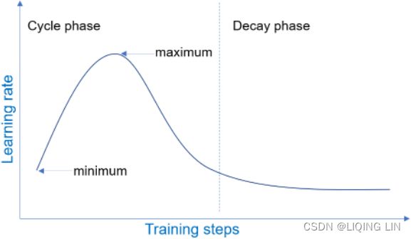 Contrary to the other approaches, 1cycle (introduced in a 2018 paper by Leslie Smith) starts by increasing the initial learning rate
 , growing linearly up to halfway through training直到训练到一半时才线性增长. Then it decreases the learning rate linearly down to again during the second half of training, finishing the last few epochs by dropping the rate down by several orders of magnitude (still linearly)学习率降低几个数量级. The maximum learning rate
 is chosen using the same approach we used to find the optimal learning rate, and the initial learning rate is chosen to be roughly 10 times lower.
When using a momentum, we start with a high momentum first (e.g., 0.95), then drop it down to a lower momentum during the first half of training (e.g., down to 0.85, linearly), and then bring it back up to the maximum value (e.g., 0.95) during the second half of training, finishing the last few epochs with that maximum value. Smith did many experiments showing that this approach was often able to speed up training considerably and reach better performance. For example, on the popular CIFAR10 image dataset, this approach reached 91.9% validation accuracy in just 100 epochs, instead of 90.3% accuracy in 800 epochs through a standard approach (with the same neural network architecture).
class OneCycleScheduler( keras.callbacks.Callback ):
def __init__(self, iterations, max_rate, start_rate=None,
last_iterations=None, last_rate=None):
self.iterations = iterations #total iterations
self.max_rate = max_rate
self.start_rate = start_rate or max_rate/10
self.last_iterations = last_iterations or iterations//10+1
self.half_iteration_pos = (iterations - self.last_iterations)//2
# finishing the last few epochs by dropping the rate down by several orders of magnitude
self.last_rate = last_rate or self.start_rate/1000
self.iteration_pos = 0
def _iterpolate( self, iter1, iter2,
rate1, rate2):
# a_slope: (rate2-rate1)/(iter2-iter1)
# x: (self.iteration-iter1)
# b: rate1
# y= a_slope * x + b
return ( (rate2-rate1)*(self.iteration_pos-iter1) / (iter2-iter1)
+ rate1 )
def on_batch_begin(self, batch, logs):
if self.iteration_pos < self.half_iteration_pos:
rate = self._iterpolate(0, self.half_iteration_pos,
self.start_rate, self.max_rate)
elif self.iteration_pos < 2*self.half_iteration_pos:
rate = self._iterpolate(self.half_iteration_pos, 2*self.half_iteration_pos,
self.max_rate, self.start_rate)
else:#last few epochs
rate = self._iterpolate(2*self.half_iteration_pos, self.iterations,
self.start_rate, self.last_rate)
self.iteration_pos +=1
K.set_value(self.model.optimizer.lr, rate)#update 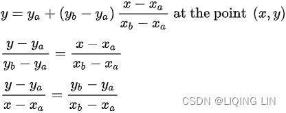 Linear interpolation
n_epochs = 15
onecycle = OneCycleScheduler( len(X_train_scaled)//batch_size*n_epochs,
                              max_rate=0.02
                            )#max_rate=0.02 from learning rate VS loss curve
history = model.fit(X_train_scaled, y_train, epochs = n_epochs, batch_size=batch_size,
                    validation_data=(X_valid_scaled, y_valid),
                    callbacks=[onecycle])
model.evaluate(X_valid_scaled, y_valid)
11_Training Deep Neural Networks_3_Adam_Learning Rate Scheduling_Decay_np.argmax(」)_lambda语句_Regular_LIQING LIN的博客-CSDN博客11_Training Deep Neural Networks_4_dropout_Max-Norm Regularization_CIFAR10_find_learning rate_LIQING LIN的博客-CSDN博客
Network architecture
The network architecture of a neural network defines its behavior. There are many forms of network architecture available; some are:
Feed forward (FF) Neural Network
A feedforward neural network (FNN) is an artificial neural network wherein connections between the nodes do not form a cycle. As such, it is different from its descendant: recurrent neural networks.
The feedforward neural network was the first and simplest type of artificial neural network devised. In this network, the information moves in only one direction—forward—from the input nodes, through the hidden nodes (if any) and to the output nodes. There are no cycles or loops in the network.
The simplest kind of neural network is a single-layer perceptron network, which consists of a single layer of output nodes; the inputs are fed directly to the outputs via a series of weights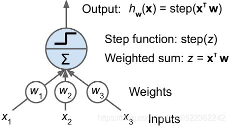 . The sum of the products of the weights and the inputs
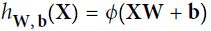 OR
OR is calculated in each node, and if the value is above some threshold (typically 0) the neuron fires and takes the activated value (typically 1); otherwise it takes the deactivated value (typically -1)
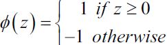 . Neurons with this kind of activation function are also called artificial neurons or linear threshold units(LTU, or called a threshold logic unit (TLU) ). In the literature the term perceptron often refers to networks consisting of just one of these units. A similar neuron was described by Warren McCulloch and Walter Pitts in the 1940s.
Figure 10-5. Architecture of a Perceptron with two input neurons, one bias neuron, and three(TLU) output neurons
Perceptron (P)
Frank Rosenblatt published the first concept of the perceptron感知器 learning rule based on the MCP(McCullock-Pitts) neuron model (F. Rosenblatt, The Perceptron, a Perceiving and Recognizing Automaton. Cornell Aeronautical Laboratory, 1957
Neurons are interconnected nerve cells in the brain that are involved in the processing and transmitting of chemical and electrical signals, which is illustrated in the following figure: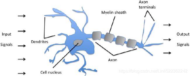 ). With his perceptron rule, Rosenblatt proposed an algorithm that would automatically learn the optimal weight coefficients that are then multiplied with the input features in order to make the decision of whether a neuron fires or not. In the context of supervised learning and classification, such an algorithm could then be used to predict if a sample belonged to one class or the other.
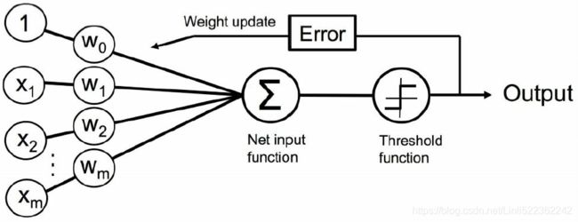
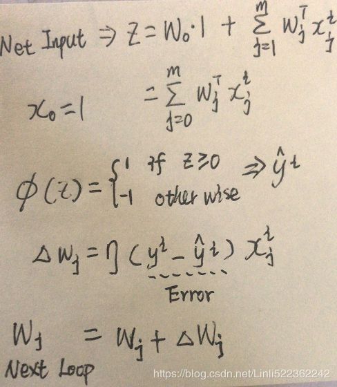 Note: Perceptron will traverse and update the weights of all feature items before entering the next loop(for next instance)
Rosenblatt's initial perceptron rule is fairly simple and can be summarized by the following steps:
- 1. Initialize the weights
 to 0 or small random numbers.
 - 2. For each training sample
 perform the following steps:
- 1.Compute the output value
 .
.
z is the Net Input:==>
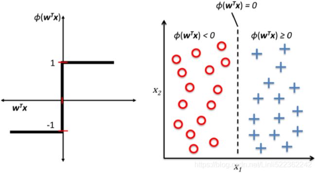
the output valueis the predicted class label predicted by the unit step function<==
 >0: the learning rate
<== <==
<==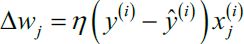 <==
<==
- 2. Update the weights.
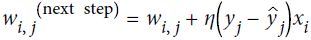
In the two scenarios where the perceptron predicts the class label correctly, the weights remain unchanged: unchanged
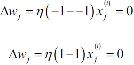
in the case of a wrong prediction, the weights are being pushed towards the direction of the positive or negative target class, respectively: increasing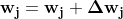 increasing
 reducing reducing
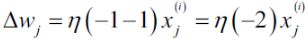 cp2_TrainingSimpleMachineLearningAlgorithmsForClassification_meshgrid_ravel_contourf_OvA_GradientDes_LIQING LIN的博客-CSDN博客
 -
class Perceptron(object):
    def __init__(self, eta =0.01, n_iter=10, random_state=1):
        self.eta = eta                   # float: Learning rate (between 0.0 and 1.0)
        self.n_iter = n_iter             # int : Passes over the training dataset
        self.random_state = random_state # int : Random number generator seed for random weight initialization.

    def fit(self, X, y): #y:Target values.      #X:shape = [n_samples, n_features]
        rgen = np.random.RandomState(self.random_state)
         #正态分布的标准差,对应分布的宽度,scale/sigma越大,正态分布的曲线越矮胖,scale越小,曲线越高瘦
                              #mu      #sigma             #n_features
        self.w_ = rgen.normal(loc=0.0, scale=0.01, size=1+X.shape[1]) #1:self.w_[0]
        #If all the weights are initialized to zero, the learning rate parameter
        #eta affects only the scale of the weight vector,

        self.errors_ = [] #Number of misclassifications (updates) in each epoch.

        for _ in range(self.n_iter):
            errors = 0
            for xi, target in zip(X,y): #xi_sample_vector, target_sample_label
                #delta_weight_vector
                update = self.eta * (target - self.predict(xi))
                # updating the weights after evaluating each individual training sample,
                # all weights += the result of (update * xi)
                self.w_[1:] += update * xi # hidden: traverse and update the weights of all features
                self.w_[0] += update
                #print(self.w_)
                errors += int(update !=0.0)
            self.errors_.append(errors)  #errors == all X_samples' error
        return self

    def net_input(self, X): # X_feature_vector * w^T
        return np.dot(X, self.w_[1:]) + self.w_[0]       #prediction=X(samples, features) dot W(features, 1)

    def predict(self, X): #X_feature_vector
        return np.where(self.net_input(X) >= 0.0, 1, -1) #classification
- 1.Compute the output value
Adaptive linear(Adaline) neurons and the convergence of learning
The key difference between the Adaline rule (also known as the Widrow-Hoff rule) and Rosenblatt's perceptron rule is that the weights are updated based on a linear activation function rather than a unit step function like in the perceptron. In Adaline, this linear activation function is simply the identity function of the net input so that
  .
.
Note: Perceptron will traverse and update the weights of all feature items before entering the next loop(for next instance) OR updating the weights incrementally after each sample) VS
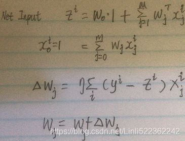 Note: the each weight update is calculated based on all samples in the training set
#OR updating the weights based on the sum of the accumulated errors over all samples xi.
Minimizing cost functions with gradient descent
One of the key ingredients of supervised machine learning algorithms is to define an objective function that is to be optimized during the learning process. This objective function is often a cost functionthat we want to minimize. In the case of Adaline, we can define the cost function to learn the weights as the Sum of Squared Errors (SSE) between the calculated outcomes and the true class labels:
 The term is just added for our convenience; it will make it easier to derive the gradient, as we will see in the following paragraphs. The main advantage of this continuous linear activation function is—in contrast to the unit step function—that the cost function becomes differentiable. Another nice property of this cost function is that it is convex; thus, we can use a simple, yet powerful, optimization algorithm called gradient descent
(https://blog.csdn.net/Linli522362242/article/details/104005906) to find the weights that minimize our cost function to classify the samples in the Iris dataset.
Using gradient descent, we can now update the weights by taking a step away from the gradient  of our cost function J(w) :
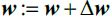
Here, the weight change is defined as the negative gradient multiplied by the learning rate
  :
: 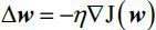
To compute the gradient of the cost function, we need to compute the partial derivative of the cost function with respect to each weight  :
: 
So that we can write the weight change as:
Since we update all weights simultaneously, our Adaline learning rule becomes ![]()
Although the Adaline learning rule looks identical to the perceptron rule, the ![]() with
with ![]() is a real number and not an integer class label. Furthermore, the each weight update is calculated based on all samples in the training set (instead of updating the weights incrementally after each sample), which is why this approach is also referred to as "batch" gradient descent.
is a real number and not an integer class label. Furthermore, the each weight update is calculated based on all samples in the training set (instead of updating the weights incrementally after each sample), which is why this approach is also referred to as "batch" gradient descent.
###############################
Note
For those who are familiar with calculus, the partial derivative of the SSE cost function with respect to the jth weight in can be obtained as follows:
###############################
Note
Performing a matrix-vector multiplication(in net_input) is similar to calculating a vector dot product where each row in the matrix is treated as a single row vector. This vectorized approach represents a more compact notation and results in a more efficient computation using NumPy. For example: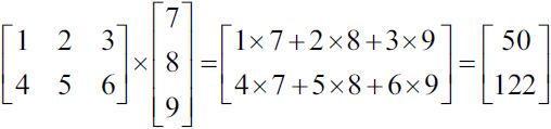
Instead of updating the weights after evaluating each individual training sample, as in the perceptron, we calculate the gradient based on the whole training dataset via self.eta * errors.sum() for the zero-weight and via self.eta * X.T.dot(errors) for the weights 1 to m where X.T.dot(errors) is a matrix-vector multiplication between our feature matrix( shape(features, samples) ) and the error vector( shape(samples,1) ). Similar to the previous perceptron implementation, we collect the cost values in a list self.cost_ to check if the algorithm converged after training.
import numpy as np

class AdalineGD(object):
    #Parameters
    # eta: Learning rate (between 0.0 and 1.0)
    # n_iter: Passes over the training dataset
    # random_state: Random number generator seed for random weight

    #Attributes
    # w_ : 1d-array # weights after fitting
    # cost_ : Sum-of-squares cost function value in each epoch
                                            #random seed
    def __init__(self, eta=0.01, n_iter=50, random_state=1):
        self.eta = eta
        self.n_iter = n_iter
        self.random_state = random_state

    def net_input(self, X):            #intercept-bradcasting along row-axis
        return np.dot(X, self.w_[1:]) + self.w_[0] # X(samples, features) dot w(features,1) + self.w_[0] ==> a single column matrix

    def activation(self, X):
        #Computer linear activation
        return X

    def fit(self, X, y): #X_array = [n_samples, n_features]
                         #y: label =[n_samples]
        rgen = np.random.RandomState(self.random_state)   #1+ n_features
        # initialization
        self.w_ = rgen.normal( loc=0.0, scale=0.01, size=1+X.shape[1] )
        self.cost_ = []

        for i in range(self.n_iter):
            net_input = self.net_input(X)     # single column matrix
            output = self.activation(net_input)       #single column matrix
            errors = (y-output) # result_vertical     #single column matrix    #rows == number of X_samples
            # update weights based on all samples in the training set
            #feature_weight
            self.w_[1:] += self.eta * X.T.dot(errors) # X.T (n_features, n_samples) #single column matrix#rows==numberOfFeatures
            self.w_[0] += self.eta * errors.sum()

            cost = (errors **2).sum() /2.0
            self.cost_.append(cost)
        return self

    def predict(self, X):
        return np.where( self.activation( self.net_input(X) )>=0.0, 1, -1 )
Note
The learning rate (eta:![]() ), as well as the number of epochs (n_iter), are the so-called hyperparameters of the perceptron and Adaline learning algorithms. In cp6_Model Eval_Confusion_Hyperpara Tuning_pipeline_variance_bias_ validation_learning curve_strength_LIQING LIN的博客-CSDN博客, Learning Best Practices for Model Evaluation and Hyperparameter Tuning, we will take a look at different techniques to automatically find the values of different hyperparameters that yield optimal performance of the classification model.
), as well as the number of epochs (n_iter), are the so-called hyperparameters of the perceptron and Adaline learning algorithms. In cp6_Model Eval_Confusion_Hyperpara Tuning_pipeline_variance_bias_ validation_learning curve_strength_LIQING LIN的博客-CSDN博客, Learning Best Practices for Model Evaluation and Hyperparameter Tuning, we will take a look at different techniques to automatically find the values of different hyperparameters that yield optimal performance of the classification model.
The Multilayer Perceptron and Backpropagation(反向传播(B-P网络),可以用来表示一种神经网络算法)
Figure 10-7. Architecture of a Multilayer Perceptron with two inputs, one hidden layer of four neurons, and three output neurons (the bias neurons are shown here, but usually they are implicit内含的)