DeepLearning学习笔记（一）：Logistic 回归

DeepLearning学习笔记（一）：Logistic 回归

  Logistic 回归是一种用于解决监督学习（Supervised Learning）问题的学习算法，其输出y的值为0或1。Logistic回归的目的是使训练数据与其预测值之间的误差最小化。
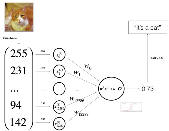
  下面以Cat vs No-cat为例： 给定以一个nx维特征向量x表示的一张图片，这个算法将估计这张图中存在一只猫的概率，即y=1的概率：
  给定 x,计算y^=P(y=1|x),且 0≤y^≤1我们希望能有一个函数，能够表示出y^，如果进行最简单的线性拟合的话，规定一个nx维向量和一个值b作为参数，可得到：

  但由于y^为一个概率值，取值范围为[0,1]，简单地进行线性拟合，得出的y^可能非常大，还可能为负值。这时，便需要一个sigmoid函数来对它的值域进行约束，sigmoid函数的表达式为：

其函数图像为：

由函数图像可知，sigmoid函数有几个很好的性质：
* 当z趋近于正无穷大时，σ(z) = 1
* 当z趋近于负无穷大时，σ(z) = 0
* 当z = 0时，σ(z) = 0.5
所以可以用sigmoid函数来约束y^的值域，此时：

成本函数

  为了训练logistic回归模型中的参数w和b，使得我们的模型输出值y^与真实值y尽可能基本一致，即尽可能准确地判断一张图是否为猫，我们需要定义一个成本函数（Cost Function）作为衡量的标准。

  用损失函数（Loss Function）来衡量预测值（y^(i)）与真实值（y(i)）之间的差异，换句话说，损失函数用来计算单个训练样本的错误。平方误差（Square Loss）是一种常用的损失函数：

  但在logistic回归中一般不使用这个损失函数，因为在训练参数过程中，使用这个损失函数将得到一个非凸函数，最终将存在很多局部最优解，这种情况下使用梯度下降（Gradient Descent）法无法找到最优解。所以在logistic回归中，一般采用log函数：

  对于一个单样本而言，误差函数L(损失函数）的定义如之前所述，而对于整体的训练集而言，用代价函数J来进行描述：

  从上式可以函数，代价函数的计算方式实际上是训练集中每个训练样本的损失函数的平均值。因此，对于一个逻辑回归问题而言，我们就是期望寻找恰当的w和b，使得最终的J尽可能的小。此时，我们可以把逻辑回归视作是一个非常小型的神经网络。

梯度下降法

  利用梯度下降法去训练w和b参数，如下图所示，假设w和b都是一个标量（Ps：实际中w是一个矢量），那么J可能取到的值是由w和b生成的曲面上的点，J的最小值，也就是对应着该曲面的底点。

  标量场中某一点上的梯度指向标量场增长最快的方向，梯度的长度是这个最大的变化率。 在空间坐标中以w，b为轴画出损失函数J(w,b)的三维图像，可知这个函数为一个凸函数。为了找到合适的参数，先将w和b赋一个初始值，正如图中的小红点。logistic回归中，通常将参数值初始化为0。梯度下降就是从起始点开始，试图在最陡峭的下降方向下坡，以便尽可能快地下坡到达最低点，这个下坡的方向便是此点的梯度值。

  以上图为例，当w位于最优点右侧时，其随着宽度的增加，高度也在不断增加，因此斜率是正数，即dw>0。因此，在迭代过程中，w的值会不断减小（w:=w-adw）。
而当w位于最优点左侧时，其随着宽度的增加，高度确在不断减小，因此斜率是负数，即dw<0。因此，在迭代过程中，w的值会不断增加（w:=w-adw）。
在实际代价函数中，J是关于w和b的函数，所以实际上，每次的迭代过程如下：

  其中的”:=“意思为赋值，α为学习率，通常为一个小于1的数，用来控制梯度下降过程中每一次移动的规格，相当于迈的步子大小。α的不宜太小也不宜过大：太小会使迭代次数增加，容易陷入局部最优解；太大容易错过最优解。

Python实现

  使用Python编写一个logistic回归分类器来识别猫，以此来了解如何使用神经网络的思维方式来进行这项任务，识别过程如图：

其中用到的Python包有：
* numpy是使用Python进行科学计算的基础包。
* matplotlib是Python中著名的绘图库。
* h5py在Python提供读取HDF5二进制数据格式文件的接口，本次的训练及测试图片集是以HDF5储存的。
* PIL(Python Image Library)为Python提供图像处理功能。
* scipy是基于NumPy来做高等数学、信号处理、优化、统计和许多其它科学任务的拓展库。

实现过程：

#导入所需要的包
import numpy as np                     #numpy：Python科学计算中最重要的库
import matplotlib.pyplot as plt        #mathplotlib：Python画图的库
import h5py                            #h5py：Python与H5文件交互的库
import scipy                           #Python科学计算相关的库
from PIL import Image                 #Python图像相关的库
from scipy import ndimage

#设置matplotlib在行内显示图片
%matplotlib inline 

 """
    # 加载数据集
    数据说明：
    对于训练集的标签而言，对于猫，标记为1，否则标记为0。
    每一个图像的维度都是(num_px, num_px, 3)，其中，长宽相同，3表示是RGB图像。
    train_set_x_orig和test_set_x_orig中，包含_orig是由于我们稍候需要对图像进行预处理，预处理后的变量将会通过
    train_dataset["train_set_x"][:] ===》命名为train_set_x和train_set_y。
    注：数据存储方式采用的是hdf5格式
"""
def load_dataset():
    train_dataset = h5py.File('datasets/train_catvnoncat.h5', "r")  #读取H5文件 读取训练数据，共209张图片
    train_set_x_orig = np.array(train_dataset["train_set_x"][:]) # your train set features 原始训练集（209*64*64*3）
    train_set_y_orig = np.array(train_dataset["train_set_y"][:]) # your train set labels  原始训练集的标签集（y=0非猫,y=1是猫）（209*1）

    test_dataset = h5py.File('datasets/test_catvnoncat.h5', "r")
    test_set_x_orig = np.array(test_dataset["test_set_x"][:]) # 原始测试集（50*64*64*3）
    test_set_y_orig = np.array(test_dataset["test_set_y"][:]) # 原始测试集的标签集（y=0非猫,y=1是猫）（50*1）

    classes = np.array(test_dataset["list_classes"][:]) # the list of classes  类别

    train_set_y_orig = train_set_y_orig.reshape((1, train_set_y_orig.shape[0]))  #对训练集和测试集标签进行reshape设为（1*209）
    test_set_y_orig = test_set_y_orig.reshape((1, test_set_y_orig.shape[0])) #原始测试集的标签集设为（1*50）
    #(1, 209)

    return train_set_x_orig, train_set_y_orig, test_set_x_orig, test_set_y_orig, classes

train_set_x_orig, train_set_y, test_set_x_orig, test_set_y, classes = load_dataset()

#print("train_set_x_orig = " + str(train_set_x_orig))
#print("train_set_y = " + str(train_set_y))
#print("test_set_x_orig = " + str(test_set_x_orig))
#print("test_set_y = " + str(test_set_y))
print("classes = " + str(classes))

classes = [b’non-cat’ b’cat’]

"""
train_set_x_orig中的每一个元素对于这一副图像，我们可以用如下代码将图像显示出来：
"""
index = 25    #index值可以改变
plt.imshow(train_set_x_orig[index])
print(train_set_y)
print(train_set_y[:, index])
print(np.squeeze(train_set_y[:, index]))
print(classes[np.squeeze(train_set_y[:, index])])
print("y = " + str(train_set_y[:, index]) + ", it's a '" + classes[np.squeeze(train_set_y[:, index])].decode("utf-8") +  "' picture.")
# y = [1], it's a 'cat' picture.

y = [1], it’s a ‘cat’ picture.

"""
接下来，我们需要根据图像集来计算出训练集的大小、测试集的大小以及图片的大小：
"""
print("train = " + str(train_set_x_orig.shape))
print("test = " + str(test_set_x_orig.shape))
print("image = " + str(train_set_x_orig.shape))
print("**************************************")
m_train = train_set_x_orig.shape[0]
m_test = test_set_x_orig.shape[0]
num_px = train_set_x_orig.shape[1]
print (m_train, m_test, num_px)
# 209, 50, 64

"""
接下来，我们需要对将每幅图像转为一个矢量，即矩阵的一列。
最终，整个训练集将会转为一个矩阵，其中包括num_px*numpy*3行，m_train列。
Ps：其中X_flatten = X.reshape(X.shape[0], -1).T可以将一个维度为(a,b,c,d)的矩阵转换为一个维度为(b∗c∗d, a)的矩阵。
"""
train_set_x_flatten = train_set_x_orig.reshape(train_set_x_orig.shape[0], -1).T
test_set_x_flatten = test_set_x_orig.reshape(test_set_x_orig.shape[0], -1).T
print(train_set_x_orig.reshape(train_set_x_orig.shape[0], -1))
print("T = " + str(train_set_x_flatten))

"""
接下来，我们需要对图像值进行归一化。
由于图像的原始值在0到255之间，最简单的方式是直接除以255即可。
"""
train_set_x = train_set_x_flatten/255.
test_set_x = test_set_x_flatten/255.

"""
接下来，我们将按照如下步骤来实现Logistic：

1. 定义模型结构

2. 初始化模型参数

3. 循环

    3.1 前向传播

    3.2 反向传递

    3.3 更新参数

4. 整合成为一个完整的模型
"""

"""
Step1：实现sigmod函数
"""
def sigmoid(z):
    """
    Compute the sigmoid of z

    Arguments:
    z -- A scalar or numpy array of any size.

    Return:
    s -- sigmoid(z)
    """
    s = 1.0 / (1 + 1 / np.exp(z))
    return s

"""
Step2：初始化参数
"""
def initialize_with_zeros(dim):
    """
    This function creates a vector of zeros of shape (dim, 1) for w and initializes b to 0.

    Argument:
    dim -- size of the w vector we want (or number of parameters in this case)

    Returns:
    w -- initialized vector of shape (dim, 1)
    b -- initialized scalar (corresponds to the bias)
    """
    w = np.zeros((dim, 1))#w为一个dim*1矩阵
    b = 0
    return w, b

"""
Step3：前向传播与反向传播
计算Y_hat,成本函数J以及dw，db
"""
def propagate(w, b, X, Y):
    """
    Implement the cost function and its gradient for the propagation explained above

    Arguments:
    w -- weights, a numpy array of size (num_px * num_px * 3, 1)
    b -- bias, a scalar
    X -- data of size (num_px * num_px * 3, number of examples)
    Y -- true "label" vector (containing 0 if non-cat, 1 if cat) of size (1, number of examples)

    Return:
    cost -- negative log-likelihood cost for logistic regression
    dw -- gradient of the loss with respect to w, thus same shape as w
    db -- gradient of the loss with respect to b, thus same shape as b

    Tips:
    - Write your code step by step for the propagation. np.log(), np.dot()
    """

    m = X.shape[1] #样本个数

    # FORWARD PROPAGATION (FROM X TO COST) 前向传播
    A = sigmoid(np.dot(w.T, X) + b)                                     # compute activation
    cost = -1 / m * np.sum(Y * np.log(A) + (1 - Y) * np.log(1 - A)) #成本函数     Y ==Y_hat   

    # BACKWARD PROPAGATION (TO FIND GRAD) 反向传播
    dw = 1 / m * np.dot(X, (A - Y).T)
    db = 1 / m * np.sum(A - Y)
    cost = np.squeeze(cost) #压缩维度    

    grads = {"dw": dw,
             "db": db} #梯度

    return grads, cost

"""
Step4：更新参数,梯度下降找出最优解
#num_iterations-梯度下降次数 learning_rate-学习率，即参数ɑ
    costs = [] #记录成本值
"""
def optimize(w, b, X, Y, num_iterations, learning_rate, print_cost = False):
    """
    This function optimizes w and b by running a gradient descent algorithm

    Arguments:
    w -- weights, a numpy array of size (num_px * num_px * 3, 1)
    b -- bias, a scalar
    X -- data of shape (num_px * num_px * 3, number of examples)
    Y -- true "label" vector (containing 0 if non-cat, 1 if cat), of shape (1, number of examples)
    num_iterations -- number of iterations of the optimization loop
    learning_rate -- learning rate of the gradient descent update rule
    print_cost -- True to print the loss every 100 steps

    Returns:
    params -- dictionary containing the weights w and bias b
    grads -- dictionary containing the gradients of the weights and bias with respect to the cost function
    costs -- list of all the costs computed during the optimization, this will be used to plot the learning curve.

    Tips:
    You basically need to write down two steps and iterate through them:
        1) Calculate the cost and the gradient for the current parameters. Use propagate().
        2) Update the parameters using gradient descent rule for w and b.
    """

    costs = []

    for i in range(num_iterations): #每次迭代循环一次， num_iterations为迭代次数


        # Cost and gradient calculation 
        grads, cost = propagate(w, b, X, Y)

        # Retrieve derivatives from grads
        dw = grads["dw"]
        db = grads["db"]

        # update rule 
        w = w - learning_rate * dw
        b = b - learning_rate * db

        # Record the costs
        if i % 100 == 0:  #每100次记录一次成本值
            costs.append(cost)

        # Print the cost every 100 training examples
        if print_cost and i % 100 == 0:   #打印成本值
            print ("Cost after iteration %i: %f" %(i, cost))
    params = {"w": w,
              "b": b}  #最终参数值
    grads = {"dw": dw,
             "db": db} #最终梯度值

    return params, grads, costs

"""
Step5：利用训练好的模型对测试集进行预测：
当输入大于0.5时，我们认为其预测认为结果是猫，否则不是猫。
"""
def predict(w, b, X):
    '''
    Predict whether the label is 0 or 1 using learned logistic regression parameters (w, b)

    Arguments:
    w -- weights, a numpy array of size (num_px * num_px * 3, 1)
    b -- bias, a scalar
    X -- data of size (num_px * num_px * 3, number of examples)

    Returns:
    Y_prediction -- a numpy array (vector) containing all predictions (0/1) for the examples in X
    '''

    m = X.shape[1] #样本个数
    Y_prediction = np.zeros((1,m)) #初始化预测输出
    w = w.reshape(X.shape[0], 1) #转置参数向量w

    # Compute vector "A" predicting the probabilities of a cat being present in the picture
    A = sigmoid(np.dot(w.T, X) + b)  #最终得到的参数代入方程

    for i in range(A.shape[1]):
        # Convert probabilities A[0,i] to actual predictions p[0,i]
        if A[0][i] > 0.5:
            Y_prediction[0][i] = 1
        else:
            Y_prediction[0][i] = 0

    return Y_prediction

"""
Step6：将以上功能整合到一个模型中：建立整个预测模型
"""
def model(X_train, Y_train, X_test, Y_test, num_iterations = 2000, learning_rate = 0.5, print_cost = False):
    """
    Builds the logistic regression model by calling the function you've implemented previously

    Arguments:
    X_train -- training set represented by a numpy array of shape (num_px * num_px * 3, m_train)
    Y_train -- training labels represented by a numpy array (vector) of shape (1, m_train)
    X_test -- test set represented by a numpy array of shape (num_px * num_px * 3, m_test)
    Y_test -- test labels represented by a numpy array (vector) of shape (1, m_test)
    num_iterations -- hyperparameter representing the number of iterations to optimize the parameters
    learning_rate -- hyperparameter representing the learning rate used in the update rule of optimize()
    print_cost -- Set to true to print the cost every 100 iterations

    Returns:
    d -- dictionary containing information about the model.
    """
    # initialize parameters with zeros 
    w, b = initialize_with_zeros(X_train.shape[0])

    # Gradient descent
    parameters, grads, costs = optimize(w, b, X_train, Y_train, num_iterations, learning_rate, print_cost) #初始化参数w，b

    # Retrieve parameters w and b from dictionary "parameters"
    w = parameters["w"]  #梯度下降找到最优参数
    b = parameters["b"]

    # Predict test/train set examples 
    Y_prediction_test = predict(w, b, X_test) #训练集的预测结果
    Y_prediction_train = predict(w, b, X_train) #测试集的预测结果

    # Print train/test Errors
    print("train accuracy: {} %".format(100 - np.mean(np.abs(Y_prediction_train - Y_train)) * 100))#训练集识别准确度
    print("test accuracy: {} %".format(100 - np.mean(np.abs(Y_prediction_test - Y_test)) * 100)) #测试集识别准确度


    d = {"costs": costs,
         "Y_prediction_test": Y_prediction_test, 
         "Y_prediction_train" : Y_prediction_train, 
         "w" : w, 
         "b" : b,
         "learning_rate" : learning_rate,
         "num_iterations": num_iterations}

    return d

"""
测试一下该模型：
"""
d = model(train_set_x, train_set_y, test_set_x, test_set_y, num_iterations = 2000, learning_rate = 0.005, print_cost = True)

Cost after iteration 0: 0.693147
Cost after iteration 100: 0.584508
Cost after iteration 200: 0.466949
Cost after iteration 300: 0.376007
Cost after iteration 400: 0.331463
Cost after iteration 500: 0.303273
Cost after iteration 600: 0.279880
Cost after iteration 700: 0.260042
Cost after iteration 800: 0.242941
Cost after iteration 900: 0.228004
Cost after iteration 1000: 0.214820
Cost after iteration 1100: 0.203078
Cost after iteration 1200: 0.192544
Cost after iteration 1300: 0.183033
Cost after iteration 1400: 0.174399
Cost after iteration 1500: 0.166521
Cost after iteration 1600: 0.159305
Cost after iteration 1700: 0.152667
Cost after iteration 1800: 0.146542
Cost after iteration 1900: 0.140872
train accuracy: 99.04306220095694 %
test accuracy: 70.0 %

"""
此时，观察打印结果，我们可以发现我们的测试准确率已经可以达到70.0%。
而对于训练集，其准确性达到了99%。这表明了我们的模型有着一定的过拟合，不过不要着急，我们会在后续的内容中来解决这一问题。

使用如下代码，我们可以挑选其中的一些图片来看我们的预测结果：
"""
# Example of a picture that was wrongly classified.
index = 8
plt.imshow(test_set_x[:,index].reshape((num_px, num_px, 3)))
print(test_set_y[0,index])
print ("y = " + str(test_set_y[0,index]) + ", you predicted that it is a \"" + 
       classes[int(d["Y_prediction_test"][0,index])].decode("utf-8") +  "\" picture.")

y = 1, you predicted that it is a “cat” picture.

"""
此外，我们还可以画出我们的代价函数变化曲线：
"""
# Plot learning curve (with costs)
costs = np.squeeze(d['costs'])
plt.plot(costs)
plt.ylabel('cost')
plt.xlabel('iterations (per hundreds)')
plt.title("Learning rate =" + str(d["learning_rate"]))
plt.show()

"""
学习速率对于最终的结果有着较大影响
分析：不同的学习速率会导致不同的预测结果。较小的学习速度收敛速度较慢，而过大的学习速度可能导致震荡或无法收敛。
"""
learning_rates = [0.01, 0.001, 0.0001]
models = {}
for i in learning_rates:
    print ("learning rate is: " + str(i))
    models[str(i)] = model(train_set_x, train_set_y, test_set_x, test_set_y, num_iterations = 1500, learning_rate = i, print_cost = False)
    print ('\n' + "-------------------------------------------------------" + '\n')

for i in learning_rates:
    plt.plot(np.squeeze(models[str(i)]["costs"]), label= str(models[str(i)]["learning_rate"]))

plt.ylabel('cost')
plt.xlabel('iterations')

legend = plt.legend(loc='upper center', shadow=True)
frame = legend.get_frame()
frame.set_facecolor('0.90')
plt.show()

learning rate is: 0.01
train accuracy: 99.52153110047847 %
test accuracy: 68.0 %

-------------------------------------------------------

learning rate is: 0.001
train accuracy: 88.99521531100478 %
test accuracy: 64.0 %

-------------------------------------------------------

learning rate is: 0.0001
train accuracy: 68.42105263157895 %
test accuracy: 36.0 %

-------------------------------------------------------

"""
用一副你自己的图像，而不是训练集或测试集中的图像
"""
## START CODE HERE ## (PUT YOUR IMAGE NAME) 
my_image = "my_image.jpg"   # change this to the name of your image file 
## END CODE HERE ##

# We preprocess the image to fit your algorithm.
fname = "images/" + my_image
image = np.array(ndimage.imread(fname, flatten=False))  #读取图片
my_image = scipy.misc.imresize(image, size=(num_px,num_px)).reshape((1, num_px*num_px*3)).T #放缩图像
my_predicted_image = predict(d["w"], d["b"], my_image)  #预测

plt.imshow(image)
print("y = " + str(np.squeeze(my_predicted_image)) + ", your algorithm predicts a \"" +
      classes[int(np.squeeze(my_predicted_image)),].decode("utf-8") +  "\" picture.")

y = 0.0, your algorithm predicts a “non-cat” picture.

参考资料

1. 吴恩达-神经网络与深度学习-网易云课堂
2. http://www.missshi.cn/#/home?_k=2uyttd
3. http://blog.csdn.net/sinat_35473930/article/details/77967260

注：本文算是博主学习DeepLearning系列课程时的学习总结吧，只是留作复习之用，并无其它意图，文中引用了其他博主的地方，也学习了很多知识，在这里表示非常感谢，水平有限，如有不妥欢迎指正。