机器学习第二十八周周报 PINNs2
文章目录
- week28 PINNs2
- 摘要
- Abstract
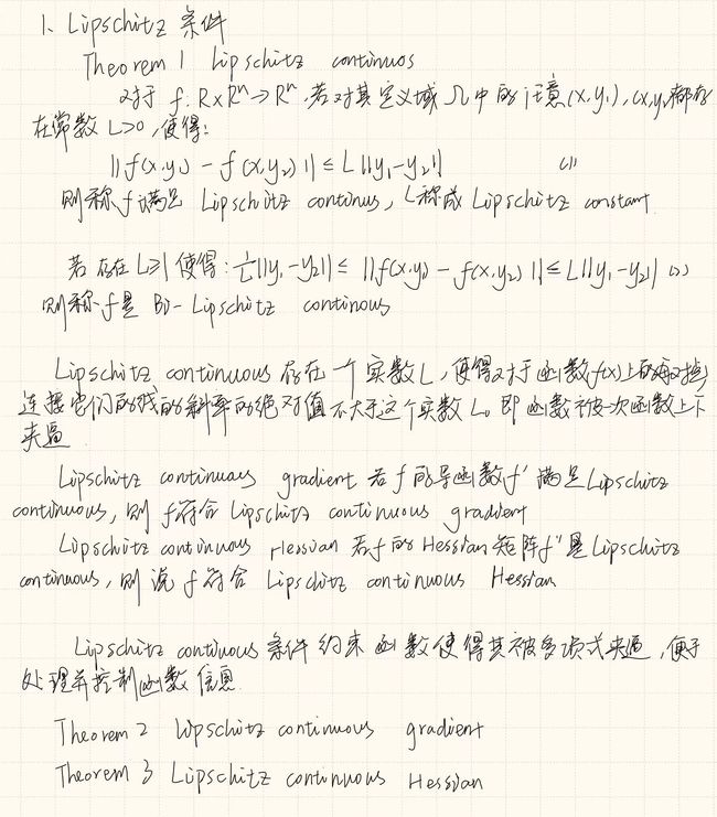
- 一、Lipschitz条件
- 二、文献阅读
-
- 1. 题目
- 数据驱动的偏微分方程
- 2. 连续时间模型
- 3. 离散时间模型
- 4.结论
- 三、CLSTM
-
- 1. 任务要求
- 2. 实验结果
- 3. 实验代码
-
- 3.1模型构建
- 3.2训练过程代码
- 小结
- 参考文献
week28 PINNs2
摘要
本文主要讨论PINN。本文简要介绍了Lipschitz条件。其次本文展示了题为Physics-informed neural networks: A deep learning framework for solving forward and inverse problems involving nonlinear partial differential equations的论文主要内容。该论文提出了一个深度学习框架,使数学模型和数据能够协同结合。该文以此为基础引出了一种有效机制,用于在较小数据规模下规范化深度神经网络的训练。该方法能够在不完整的模型以及数据中推测出较为合理的结果。本文主要集中在该文第四节——数据驱动的偏微分方程。最后,本文基于pytorch实现了CLSTM并使用序列数据训练该模型。
Abstract
This article focuses on PINN. This article provides a brief introduction to the Lipschitz condition. Secondly, this article presents the main content of the paper entitled Physics-informed neural networks: A deep learning framework for solving forward and inverse problems involving nonlinear partial differential equations. The paper proposes a deep learning framework that enables mathematical models and data to be synergistically combined. Based on this, this paper proposes an effective mechanism for the training of normalized deep neural networks at a small data scale. This method can infer reasonable results from incomplete models and data. This paper focuses on Section 4 of the paper, Data-driven discovery of partial differential equations. Finally, this article implements CLSTM based on pytorch and trains the model with sequential data.
一、Lipschitz条件
二、文献阅读
1. 题目
题目:Physics-informed neural networks: A deep learning framework for solving forward and inverse problems involving nonlinear partial differential equations
作者:M. Raissi, P. Perdikaris , G.E. Karniadakis
链接:https://www.sciencedirect.com/science/article/pii/S0021999118307125
发布:Journal of Computational Physics Volume 378, 1 February 2019, Pages 686-707
数据驱动的偏微分方程
本篇为该论文的第二部分,第一部分已经在上周周报中进行阐述。而在离散时间模型中的龙格库塔方法在上文中从一二阶进行了完整的推导,并给出了四阶龙格库塔的形式
注:正如上篇周报中一样,由于其实验在阐述模型的具体形式后给出,因此不再单独阐述实验。
该问题同样有两种不同类型的算法,即连续时间模型以及离散时间模型。
2. 连续时间模型
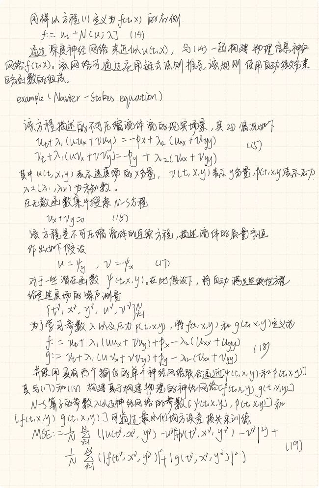

为了针对该问题生成高分辨率数据集,采用spectral/hp-element求解器NekTar。
具体来说,解域通过由 412 个三角形元素组成的曲面细分在空间中离散化,并且在每个元素内,解近似为十阶分层半正交雅可比多项式展开的线性组合。假设在左边界处施加均匀的自由流速度分布,在位于圆柱体下游 25 个直径的右边界处施加零压力流出条件,以及 [−15, 25] × 的顶部和底部边界的周期性[−8, 8] 域。使用三阶刚性稳定方案对方程(15)进行积分,直到系统达到周期性稳态,如下图(a)所示。接下来,与该稳态解相对应的结果数据集的一小部分将用于模型训练,而其余数据将用于验证预测。

给定流向 u(t, x, y) 和横向 v(t, x, y) 速度分量上的分散且潜在噪声的数据,目标是识别未知参数 λ1 和 λ2,并获得定性准确地重建气缸尾流中的整个压力场 p(t, x, y),根据定义只能识别一个常数。通过对完整高分辨率数据集进行随机子采样来创建训练数据集。
为了强调该方法从分散和稀缺的训练数据中学习的能力,选择 N = 5,000,仅相当于可用数据总数的 1%,如上图(b)所示。
使用的神经网络架构由 9 层组成,每层 20 个神经元。
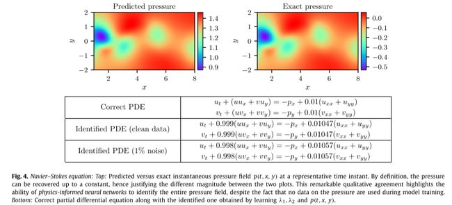
如下图,即使训练数据被噪声破坏,物理信息神经网络也能够以非常高的精度正确识别未知参数 λ1 和 λ2。具体来说,对于无噪声训练数据的情况,估计λ1和λ2的误差分别为0.078%和4.67%。即使训练数据被 1% 的不相关高斯噪声破坏,预测仍然保持稳健,对于 λ1 和 λ2 分别返回 0.17% 和 5.70% 的误差。
下图展示了代表性压力快照与精确压力解的视觉比较。通过利用基础物理学从辅助测量中推断出连续的变量的物理信息神经网络能够较好的拟合参数,并凸显了其在解决高维逆问题方面的潜力。
3. 离散时间模型

example:(Korteweg–de Vries 方程):以下简称KdV方程
KdV 方程为
u t + λ 1 u u x + λ 2 u x x x = 0 (27) u_t+\lambda_1uu_x+\lambda_2u_{xxx}=0 \tag{27} ut+λ1uux+λ2uxxx=0(27)
其中 (λ1, λ2) 为未知参数。
对于 KdV 方程,方程 (22) 中的非线性算子形式为
N [ u n + c j ] = λ 1 u n + c j − λ 2 u x x x n + c \mathcal N[u^{n+c_j}]=\lambda_1u^{n+c_j}-\lambda_2u_{xxx}^{n+c} N[un+cj]=λ1un+cj−λ2uxxxn+c
并由该式同神经网络(23)、(24)的共享参数共同给出,和(25)以及KdV方程的参数 λ = ( λ 1 , λ 2 ) \lambda=(\lambda_1,\lambda_2) λ=(λ1,λ2)
KdV 方程的值可以通过最小化误差平方和(26)来学习
从初始条件 u(0, x) = cos(πx) 开始并假设周期性边界条件,使用带有谱傅里叶的 Chebfun 包将方程 (27) 积分到最终时间 t = 1.0使用 512 个模式和时间步长 t = 1 0 − 6 t = 10^{−6} t=10−6 的四阶显式龙格-库塔时间积分器进行离散化。使用该数据集,在时间 t n = 0.2 t_n = 0.2 tn=0.2 和 t n + 1 = 0.8 t_{n+1} = 0.8 tn+1=0.8 时提取两个解的快照,并使用 N n = 199 N_n = 199 Nn=199 和 N n + 1 = 201 N_{n+1} = 201 Nn+1=201 对它们进行随机子采样以生成训练数据集。然后,使用 L-BFGS 最小化方程 (26) 的误差平方和损失,从而使用这些数据来训练离散时间物理信息神经网络。这里使用的网络架构由 4 个隐藏层、每层 50 个神经元和一个输出层组成,该输出层预测 q 个 Runge-Kutta 阶段的解,即 u n + c j ( x ) , j = 1 , . . . , q u^{n+c_j(x)}, j = 1, ..., q un+cj(x),j=1,...,q,其中 q 是根据经验选择的,通过设置产生机器精度量级的时间误差累积
q = 0.5 log ϵ / log ( Δ t ) (28) q=0.5\log\epsilon/\log(\Delta t) \tag{28} q=0.5logϵ/log(Δt)(28)
在本例中 Δ t = 0.6 \Delta t=0.6 Δt=0.6
上图总结了该实验的结果。在顶部面板中,展示了精确的解 u ( t , x ) u(t, x) u(t,x)以及用于训练的两个数据快照的位置。中间面板给出了精确解决方案和训练数据的更详细概述。值得注意的是,方程(27)的复杂非线性动力学如何导致两个报告快照之间的解形式存在巨大差异。尽管存在这些差异,并且两个训练快照之间存在较大的时间间隙,但无论训练数据是否被噪声损坏,该方法都能够正确识别未知参数。具体来说,对于无噪声训练数据的情况,估计 λ 1 和 λ 2 λ_1 和 λ_2 λ1和λ2 的误差分别为 0.023% 和 0.006%,而训练数据中有 1% 噪声的情况返回误差分别为 0.057% 和 0.017%。

4.结论
该文引入了了基于物理的神经网络,这是一类新型的通用函数逼近器,能够对控制给定数据集的任何基本物理定律进行编码,并且可以通过偏微分方程进行描述。其设计了数据驱动算法,用于推断一般非线性偏微分方程的解,并构建计算高效的物理信息替代模型。由此产生的方法为计算科学中的各种问题展示了一系列有希望的结果,并为赋予深度学习强大的数学物理能力来模拟周围的世界开辟了道路。
三、CLSTM
本网络框架由该文章提出。该文章提出的C-LSTM 利用 CNN 提取一系列更高级别的表示,并将其输入到长短期记忆循环神经网络 (LSTM) 中以获得全局表示。C-LSTM能够捕获短语的局部特征以及全局和时间信息。该文章评估了所提出的关于情感分类和问题分类任务的架构。实验结果表明,C-LSTM的性能优于CNN和LSTM,可以在这些任务上取得优异的性能。
1. 任务要求
本文实现了上述网络结构,并使用从网络上爬取的序列信息作为数据集进行训练,详情参照第25周周报,故本文不再给出这部分内容相关解释。
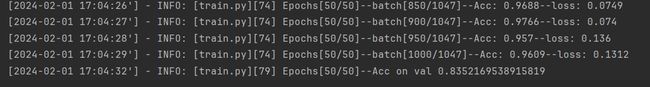
2. 实验结果
训练结果如下:
3. 实验代码
3.1模型构建
"""
Zhou C, Sun C, Liu Z, et al. A C-LSTM neural network for text classification[J]. arXiv preprint arXiv:1511.08630, 2015.
"""
import torch.nn as nn
import torch


class CLSTM(nn.Module):
    def __init__(self, config):
        super(CLSTM, self).__init__()
        if config.cell_type == 'RNN':
            rnn_cell = nn.RNN
        elif config.cell_type == 'LSTM':
            rnn_cell = nn.LSTM
        elif config.cell_type == 'GRU':
            rnn_cell = nn.GRU
        else:
            raise ValueError("Unrecognized RNN cell type: " + config.cell_type)
        out_hidden_size = config.hidden_size * (int(config.bidirectional) + 1)
        self.config = config
        self.token_embedding = nn.Embedding(config.vocab_size, config.embedding_size)
        self.conv = nn.Conv2d(1, config.out_channels,
                              kernel_size=(config.window_size, config.embedding_size))
        self.rnn = rnn_cell(config.out_channels, config.hidden_size, config.num_layers,
                            batch_first=True, bidirectional=config.bidirectional)
        self.classifier = nn.Sequential(nn.Linear(out_hidden_size, config.num_classes))

    def forward(self, x, labels=None):
        """
        :param x: [batch_size, src_len]
        :param labels: [batch_size]
        :return:
        """
        x = self.token_embedding(x)  # [batch_size, src_len, embedding_size]
        x = torch.unsqueeze(x, dim=1)  # [batch_size, 1, src_len, embedding_size]
        feature_maps = self.conv(x).squeeze(-1)  # [batch_size, out_channels, src_len-window_size+1]
        feature_maps = feature_maps.transpose(1, 2)  # [batch_size, src_len-window_size+1, out_channels]
        x, _ = self.rnn(feature_maps)  # [batch_size, src_len-window_size+1, out_hidden_size]
        if self.config.cat_type == 'last':
            x = x[:, -1]  # [batch_size, out_hidden_size]
        elif self.config.cat_type == 'mean':
            x = torch.mean(x, dim=1)  # [batch_size, out_hidden_size]
        elif self.config.cat_type == 'sum':
            x = torch.sum(x, dim=1)  # [batch_size, out_hidden_size]
        else:
            raise ValueError("Unrecognized cat_type: " + self.cat_type)
        logits = self.classifier(x)  # [batch_size, num_classes]
        if labels is not None:
            loss_fct = nn.CrossEntropyLoss(reduction='mean')
            loss = loss_fct(logits, labels)
            return loss, logits
        else:
            return logits


class ModelConfig(object):
    def __init__(self):
        self.num_classes = 15
        self.vocab_size = 8
        self.embedding_size = 16
        self.out_channels = 32
        self.window_size = 3
        self.hidden_size = 128
        self.num_layers = 1
        self.cell_type = 'LSTM'
        self.bidirectional = False
        self.cat_type = 'last'


if __name__ == '__main__':
    config = ModelConfig()
    model = CLSTM(config)
    x = torch.randint(0, config.vocab_size, [2, 10], dtype=torch.long)
    label = torch.randint(0, config.num_classes, [2], dtype=torch.long)
    loss, logits = model(x, label)
    print(loss)
    print(logits)
3.2训练过程代码
from transformers import optimization
from torch.utils.tensorboard import SummaryWriter
import torch
from copy import deepcopy
import sys
import logging
import os
from CLSTM import CLSTM

sys.path.append("../../")
from utils import TouTiaoNews


class ModelConfig(object):
    def __init__(self):
        self.batch_size = 256
        self.epochs = 50
        self.learning_rate = 6e-4
        self.num_classes = 15
        self.vocab_size = 3000
        self.embedding_size = 256
        self.out_channels = 256  # input_dim
        self.window_size = 3  # cnn filter size
        self.hidden_size = 256  # rnn_hidden_size
        self.num_layers = 1
        self.cell_type = 'LSTM'
        self.bidirectional = True
        self.cat_type = 'last'
        self.num_warmup_steps = 200
        self.model_save_path = 'model.pt'
        self.summary_writer_dir = "runs/model"
        self.device = torch.device('cuda:0' if torch.cuda.is_available() else 'cpu')
        # 判断是否存在GPU设备,其中0表示指定第0块设备
        logging.info("### 将当前配置打印到日志文件中 ")
        for key, value in self.__dict__.items():
            logging.info(f"### {key} = {value}")


def train(config):
    toutiao_news = TouTiaoNews(top_k=config.vocab_size,
                               batch_size=config.batch_size,
                               cut_words=False)
    train_iter, val_iter = toutiao_news.load_train_val_test_data(is_train=True)
    model = CLSTM(config)
    if os.path.exists(config.model_save_path):
        logging.info(f" # 载入模型{config.model_save_path}进行追加训练...")
        checkpoint = torch.load(config.model_save_path)
        model.load_state_dict(checkpoint)
    optimizer = torch.optim.Adam(model.parameters(), lr=config.learning_rate)
    writer = SummaryWriter(config.summary_writer_dir)
    model = model.to(config.device)
    max_test_acc = 0
    steps = len(train_iter) * config.epochs
    scheduler = optimization.get_cosine_schedule_with_warmup(optimizer, num_warmup_steps=config.num_warmup_steps,
                                                             num_training_steps=steps, num_cycles=2)
    for epoch in range(config.epochs):
        for i, (x, y) in enumerate(train_iter):
            x, y = x.to(config.device), y.to(config.device)
            loss, logits = model(x, y)
            optimizer.zero_grad()
            loss.backward()
            optimizer.step()  # 执行梯度下降
            scheduler.step()
            if i % 50 == 0:
                acc = (logits.argmax(1) == y).float().mean()
                logging.info(f"Epochs[{epoch + 1}/{config.epochs}]--batch[{i}/{len(train_iter)}]"
                             f"--Acc: {round(acc.item(), 4)}--loss: {round(loss.item(), 4)}")
                writer.add_scalar('Training/Accuracy', acc, scheduler.last_epoch)
            writer.add_scalar('Training/Loss', loss.item(), scheduler.last_epoch)
        test_acc = evaluate(val_iter, model, config.device)
        logging.info(f"Epochs[{epoch + 1}/{config.epochs}]--Acc on val {test_acc}")
        writer.add_scalar('Testing/Accuracy', test_acc, scheduler.last_epoch)
        if test_acc > max_test_acc:
            max_test_acc = test_acc
            state_dict = deepcopy(model.state_dict())
            torch.save(state_dict, config.model_save_path)


def evaluate(data_iter, model, device):
    model.eval()
    with torch.no_grad():
        acc_sum, n = 0.0, 0
        for x, y in data_iter:
            x, y = x.to(device), y.to(device)
            logits = model(x)
            acc_sum += (logits.argmax(1) == y).float().sum().item()
            n += len(y)
        model.train()
        return acc_sum / n


def inference(config, test_iter):
    model = CLSTM(config)
    model.to(config.device)
    model.eval()
    if os.path.exists(config.model_save_path):
        logging.info(f" # 载入模型进行推理……")
        checkpoint = torch.load(config.model_save_path)
        model.load_state_dict(checkpoint)
    else:
        raise ValueError(f" # 模型{config.model_save_path}不存在!")
    first_batch = next(iter(test_iter))
    with torch.no_grad():
        logits = model(first_batch[0].to(config.device))
    y_pred = logits.argmax(1)
    logging.info(f"真实标签为:{first_batch[1]}")
    logging.info(f"预测标签为:{y_pred}")


if __name__ == '__main__':
    config = ModelConfig()
    train(config)

    #   推理
    # toutiao_news = TouTiaoNews(top_k=config.vocab_size,
    #                            batch_size=config.batch_size,
    #                            cut_words=False)
    # test_iter = toutiao_news.load_train_val_test_data(is_train=False)
    # inference(config, test_iter)
小结
本文简要了解了Lipschitz条件,下周将继续学习MLP上的Lipshchitz条件并证明其是NP问题。
本文简要介绍了PINN,讨论了方面,在连续时间模型上使用NS方程验证模型,在离散时间模型上使用Korteweg–de Vries 方程验证模型,均表现出了较好的效果。下周将继续阅读序列化相关文章。
参考文献
[1] M. Raissi a, et al. “Physics-Informed Neural Networks: A Deep Learning Framework for Solving Forward and Inverse Problems Involving Nonlinear Partial Differential Equations.” Journal of Computational Physics, Academic Press, 3 Nov. 2018, www.sciencedirect.com/science/article/pii/S0021999118307125.
[2] Zhou C, Sun C, Liu Z, et al. A C-LSTM neural network for text classification[J]. arXiv preprint arXiv:1511.08630, 2015