深度学习(13)--搭建神经网络进行气温预测

一.搭建神经网络进行气温预测流程详解

1.1.导入所需的工具包

import numpy as np  # 矩阵计算
import pandas as pd   # 数据读取
import matplotlib.pyplot as plt  # 画图处理
import torch  # 构建神经网络
import torch.optim as optim  # 设置优化器

1.2.读取并处理数据

引入数据并查看数据的格式

# 引入数据
features = pd.read_csv('temps.csv')

# 看看数据长什么样子
print(features.head())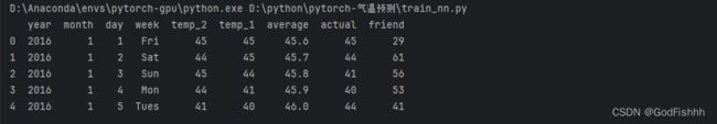

Pandas库中的.head()函数，取数据的前n行数据，默认是取前五行数据，如上图所示。

查看数据维度

print('数据维度:', features.shape)

shape函数的功能是读取矩阵的长度，.shape直接输出数据的维度，如上图，表示该数据的维度为348行，9列。对应的也就是348个样本，9个特征。

而shape[0]，shape[1]则分别返回矩阵第一维度、第二维度的长度：

# 查看数据维度
print('数据维度:', features.shape[0])
print('数据维度:', features.shape[1])

处理时间数据

# 处理时间数据
import datetime

# 分别得到年，月，日
years = features['year']
months = features['month']
days = features['day']

# datetime格式
dates = [str(int(year)) + '-' + str(int(month)) + '-' + str(int(day)) for year, month, day in zip(years, months, days)]
dates = [datetime.datetime.strptime(date, '%Y-%m-%d') for date in dates]

 查看处理的datas数据格式

print(dates[:3])

对特殊数据进行one-hot编码 

计算机无法识别字符串数据，所以对于字符串数据需要使用one-hot编码：

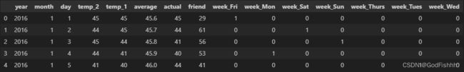
features = pd.get_dummies(features) 

# get_dummies会自动判断数据中哪一列是字符串，并自动将字符串展开。

# eg:数据中用于标注星期的字符串一共有七个，则get_dummies函数将数据展开成七列，当天是哪一天就在相应位置标1。

# 星期 一 二 三 四 五 六 七，如果是星期一则标注为：1 0 0 0 0 0 0，如果是星期三则标注为：0 0 1 0 0 0 0，如果是星期六则标注为：0 0 0 0 0 1 0

 查看one-hot编码后的数据

对标签进行处理

# 标签
labels = np.array(features['actual'])  # 获取标签：features获取actual的标签然后再转换为np.array的格式

# 在特征中去掉标签
features= features.drop('actual', axis = 1)  # 去除features中的actual标签，axis表示沿着行/列去除，axis=0按行计算，axis=1按列计算

# 名字单独保存一下，以备后患
feature_list = list(features.columns)  # 保存features中的columns值，也就是列

# 转换成合适的格式
features = np.array(features)  # 把处理后的features数据也转换为np.array格式

 

标准化处理 

不同的数据取值范围不同，而机器又会认为数值大的数据较为重要，所以需要对数据进行标准化(x-μ/σ) -- μ为均值，σ为标准差。

from sklearn import preprocessing
input_features = preprocessing.StandardScaler().fit_transform(features)  # fit_transform通过数据计算出均值和标准差，再对数据进行标准化处理变换。

fit_transform通过数据计算出均值和标准差，再对数据进行标准化处理变换。

标准化处理前后的数据：

1.3.构建网络模型

构建网络

本项目构建的网络模型较为简单，只有一个隐层

# shape[0]是样本数，也就是行的数据，shape[1]是特征数，也就是列的数据
input_size = input_features.shape[1]  
hidden_size = 128
output_size = 1
batch_size = 16  # 一次迭代batch个样本
my_nn = torch.nn.Sequential(
    torch.nn.Linear(input_size, hidden_size),  # 根据输入自动初始化权重参数和偏重值
    torch.nn.ReLU(),  # 激活函数 Sigmoid/Relu
    torch.nn.Linear(hidden_size, output_size),
)
cost = torch.nn.MSELoss(reduction='mean')  # 损失函数设置：MSE均方误差
optimizer = torch.optim.Adam(my_nn.parameters(), lr=0.001)  
# 优化器设置：Adam，参数为网络中的所有参数以及学习率

训练网络

# 训练网络
losses = []
# 迭代1000次,epoch = 1000
for i in range(1000):
    batch_loss = []
    # MINI-Batch方法来进行训练
    for start in range(0, len(input_features), batch_size):  # 循环范围为0~样本数，每次循环中间间隔batchs_size
        end = start + batch_size if start + batch_size < len(input_features) else len(input_features)  # 做一个索引是否越界的判断
        # 取得一个batch的数据
        xx = torch.tensor(input_features[start:end], dtype = torch.float, requires_grad = True)
        yy = torch.tensor(labels[start:end], dtype = torch.float, requires_grad = True)
        prediction = my_nn(xx)  # 输入值经过定义的网络运算得到预测值
        loss = cost(prediction, yy)  # 参数为预测值和真实值
        optimizer.zero_grad()  # torch的迭代过程中会累计之前的训练结果，所以在每次迭代中需要清空梯度值
        loss.backward(retain_graph=True)  # 反向传播
        optimizer.step()  # 对所有参数进行更新
        batch_loss.append(loss.data.numpy())
    
    # 打印损失
    if i % 100==0:
        losses.append(np.mean(batch_loss))
        print(i, np.mean(batch_loss))

预测训练结果 

x = torch.tensor(input_features, dtype = torch.float)  
# 先将数据转换为tensor格式，因为需要在网络中进行运算
predict = my_nn(x).data.numpy()  
# 在网络中运算完成中，再转换为data.numpy格式，因为后续需要进行画图处理

1.4.对结果进行画图对比

# 转换日期格式
dates = [str(int(year)) + '-' + str(int(month)) + '-' + str(int(day)) for year, month, day in zip(years, months, days)]
dates = [datetime.datetime.strptime(date, '%Y-%m-%d') for date in dates]

# 创建一个表格来存日期和其对应的标签数值
true_data = pd.DataFrame(data={'date': dates, 'actual': labels})

# 同理，再创建一个来存日期和其对应的模型预测值
months = features[:, feature_list.index('month')]
days = features[:, feature_list.index('day')]
years = features[:, feature_list.index('year')]

test_dates = [str(int(year)) + '-' + str(int(month)) + '-' + str(int(day)) for year, month, day in zip(years, months, days)]
test_dates = [datetime.datetime.strptime(date, '%Y-%m-%d') for date in test_dates]

predictions_data = pd.DataFrame(data = {'date': test_dates, 'prediction': predict.reshape(-1)})   # predict是x经过网络训练再转换为np.array的值

# 画图

# 真实值
plt.plot(true_data['date'], true_data['actual'], 'b-', label='actual')  # 参数分别为：横轴，纵轴，曲线颜色，标签值

# 预测值
plt.plot(predictions_data['date'], predictions_data['prediction'], 'ro', label='prediction')  # 参数分别为：横轴，纵轴，曲线颜色，标签值
plt.xticks(rotation=30)  # x轴参数倾斜60°
plt.legend()  # 使上述代码产生效果

# 图名
plt.xlabel('Date')
plt.ylabel('Maximum Temperature (F)')  # x,y轴标签设置
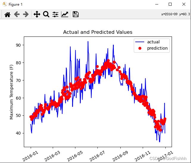
plt.title('Actual and Predicted Values')  # 图名设置

# 保存图片并展示
plt.savefig("result.png")
plt.show()

二.完整代码

import numpy as np  # 矩阵计算
import pandas as pd   # 数据读取
import matplotlib.pyplot as plt  # 画图处理
import torch  # 构建神经网络
import torch.optim as optim  # 设置优化器

# 处理时间数据
import datetime

from sklearn import preprocessing

# 引入数据
features = pd.read_csv('temps.csv')

# 看看数据长什么样子
# print(features.head())

# 查看数据维度
# print('数据维度:', features.shape)


# 分别得到年，月，日
years = features['year']
months = features['month']
days = features['day']

'''
# datetime格式
dates = [str(int(year)) + '-' + str(int(month)) + '-' + str(int(day)) for year, month, day in zip(years, months, days)]
dates = [datetime.datetime.strptime(date, '%Y-%m-%d') for date in dates]

print(dates[:3])
'''

# 独热(one-hot)编码 -- 机器不认识字符串，需要将字符串转换为机器认识的参数
features = pd.get_dummies(features)
# get_dummies会自动判断数据中哪一列是字符串，并自动将字符串展开
# eg:数据中用于标注星期的字符串一共有七个，则get_dummies函数将数据展开成七列，当天是哪一天就在相应位置标1
# 星期 一 二 三 四 五 六 七，如果是星期一则标注为：1 0 0 0 0 0 0，如果是星期三则标注为：0 0 1 0 0 0 0，如果是星期六则标注为：0 0 0 0 0 1 0
# print(features.head(5))

# 标签
labels = np.array(features['actual'])  # 获取标签：features获取actual的标签然后再转换为np.array的格式

# 在特征中去掉标签
features = features.drop('actual', axis = 1)  # 去除features中的actual标签，axis表示沿着行/列去除，axis=0按行计算，axis=1按列计算

# 名字单独保存一下，以备后患
feature_list = list(features.columns)  # 保存features中的columns值，也就是列

# 转换成合适的格式
features = np.array(features)  # 把处理后的features数据也转换为np.array格式

# print(features[0])
# 标准化处理
input_features = preprocessing.StandardScaler().fit_transform(features)
# fit_transform通过数据计算出均值和标准差，再对数据进行标准化处理变换。
# print(input_features[0])

# shape[0]是样本数，也就是行的数据，shape[1]是特征数，也就是列的数据
input_size = input_features.shape[1]
hidden_size = 128
output_size = 1
batch_size = 16  # 一次迭代batch个样本
my_nn = torch.nn.Sequential(
    torch.nn.Linear(input_size, hidden_size),  # 根据输入自动初始化权重参数和偏重值
    torch.nn.ReLU(),  # 激活函数 Sigmoid/ReLU
    torch.nn.Linear(hidden_size, output_size),
)
cost = torch.nn.MSELoss(reduction='mean')  # 损失函数设置：MSE均方误差
optimizer = torch.optim.Adam(my_nn.parameters(), lr=0.001)
# 优化器设置：Adam，参数为网络中的所有参数以及学习率

# 训练网络
losses = []
# 迭代1000次,epoch = 1000
for i in range(1000):
    batch_loss = []
    # MINI-Batch方法来进行训练
    for start in range(0, len(input_features), batch_size):  # 循环范围为0~样本数，每次循环中间间隔batchs_size
        end = start + batch_size if start + batch_size < len(input_features) else len(input_features)  # 做一个索引是否越界的判断
        # 取得一个batch的数据
        xx = torch.tensor(input_features[start:end], dtype=torch.float, requires_grad=True)
        yy = torch.tensor(labels[start:end], dtype=torch.float, requires_grad=True)
        prediction = my_nn(xx)  # 输入值经过定义的网络运算得到预测值
        loss = cost(prediction, yy)  # 参数为预测值和真实值
        optimizer.zero_grad()  # torch的迭代过程中会累计之前的训练结果，所以在每次迭代中需要清空梯度值
        loss.backward(retain_graph=True)  # 反向传播
        optimizer.step()  # 对所有参数进行更新
        batch_loss.append(loss.data.numpy())

    '''
    # 打印损失
    if i % 100 == 0:
        losses.append(np.mean(batch_loss))
        print(i, np.mean(batch_loss))
    '''

# 预测训练结果
x = torch.tensor(input_features, dtype=torch.float)
# 先将数据转换为tensor格式，因为需要在网络中进行运算
predict = my_nn(x).data.numpy()
# 在网络中运算完成中，再转换为data.numpy格式，因为后续需要进行画图处理

# 转换日期格式
dates = [str(int(year)) + '-' + str(int(month)) + '-' + str(int(day)) for year, month, day in zip(years, months, days)]
dates = [datetime.datetime.strptime(date, '%Y-%m-%d') for date in dates]

# 创建一个表格来存日期和其对应的标签数值
true_data = pd.DataFrame(data={'date': dates, 'actual': labels})

# 同理，再创建一个来存日期和其对应的模型预测值
months = features[:, feature_list.index('month')]
days = features[:, feature_list.index('day')]
years = features[:, feature_list.index('year')]

test_dates = [str(int(year)) + '-' + str(int(month)) + '-' + str(int(day)) for year, month, day in zip(years, months, days)]
test_dates = [datetime.datetime.strptime(date, '%Y-%m-%d') for date in test_dates]

predictions_data = pd.DataFrame(data = {'date': test_dates, 'prediction': predict.reshape(-1)})   # predict是x经过网络训练再转换为np.array的值

# 画图

# 真实值
plt.plot(true_data['date'], true_data['actual'], 'b-', label='actual')  # 参数分别为：横轴，纵轴，曲线颜色，标签值

# 预测值
plt.plot(predictions_data['date'], predictions_data['prediction'], 'ro', label='prediction')  # 参数分别为：横轴，纵轴，曲线颜色，标签值
plt.xticks(rotation=30)  # x轴参数倾斜60°
plt.legend()  # 使上述代码产生效果

# 图名
plt.xlabel('Date')
plt.ylabel('Maximum Temperature (F)')  # x,y轴标签设置
plt.title('Actual and Predicted Values')  # 图名设置

# 保存图片并展示
plt.savefig("result.png")
plt.show()

三.输出结果