PyTorch深度学习实战（34）——Pix2Pix详解与实现

0. 前言

Pix2Pix 是基于生成对抗网络 (Convolutional Generative Adversarial Networks, GAN) 的图像转换框架，能够将输入图像转换为与之对应的输出图像，能够广泛用于图像到图像转换的任务，如风格转换、图像修复、语义标签到图像的转换等。Pix2Pix 的核心思想是通过对抗训练将输入图像和目标输出图像进行配对，使生成网络可以学习到输入图像到输出图像的映射关系。在本节中，将学习使用 Pix2Pix 根据给定轮廓生成图像。

1. 模型与数据集

1.1 Pix2Pix 基本原理

Pix2Pix 是基于对抗生成网络 (Convolutional Generative Adversarial Networks, GAN) 的图像转换算法，可以将一种图像转换为与之对应的输出图像。例如，将黑白线稿转换为彩色图像或将低分辨率图像转换为高分辨率图像等。Pix2Pix 已经被广泛应用于计算机视觉领域，例如风格迁移、语义分割、图像去雾等任务。
假设，数据集中包含成对的相互关联图像，例如，线稿图像作为输入，实际图像作为输出。如果我们要在给定线稿输入图像的情况下生成图像，传统方法中，可以将其视为输入到输出的简单映射(即监督学习问题)，但传统监督学习只能从历史数据中学习，无法为新线稿生成逼真图像。而 GAN 能够在确保生成的图像足够逼真的情况下，为新数据样本输出合理预测结果。

1.2 数据集分析

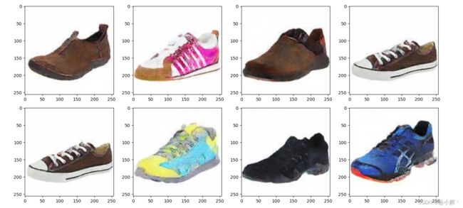
为了训练 Pix2Pix 模型，我们需要了解本节所用的数据集，数据集取自 berkeley Pix2Pix 数据集，可以自行构建数据集，也可以下载本文所用数据集，下载地址：https://pan.baidu.com/s/1a7VE-z1mGWhbIvvst9e8Ng，提取码：rkvd。数据集包含 4381 张不同样式和颜色的鞋子照片，图像尺寸为 256 x 256。

1.3 模型构建策略

在本节中，我们将构建 PixPix 模型，根据鞋子的手绘轮廓生成鞋子图像，模型构建策略如下：

• 获取实际图像并使用 cv2 边缘检测技术创建相应的物体轮廓
• 从原始图像的区块中提取颜色样本，以便生成网络预测所需生成的颜色
• 构建 UNet 架构作为生成网络，将带有样本区块颜色的轮廓作为输入并预测相应的图像
• 构建判别网络架构，获取输入图像并预测它是真实图像还是生成图像
• 训练生成网络和判别网络，直到生成网络可以生成欺骗判别网络的生成图像

2. 实现 Pix2Pix 生成图像

接下来，使用 PyTorch 实现 Pix2Pix 模型，根据给定鞋子轮廓生成图像。

(1) 导入数据集以及所需库：

import torch
from torch import nn
from torch import optim
from matplotlib import pyplot as plt
import numpy as np
from torchvision.utils import make_grid
from torch.utils.data import DataLoader, Dataset
import cv2
import random
from glob import glob
# from torch_snippets import *
device = "cuda" if torch.cuda.is_available() else "cpu"

from torchvision import transforms

下载后的图像示例如下：

在本节中，我们需要在给定轮廓(边缘)和鞋子的区块颜色的情况下绘制鞋子。接下来，获取给定鞋子图像的边缘，然后训练模型，根据给定鞋子的轮廓和区块颜色重建鞋子图像。

(2) 定义函数，用于从图像中获取边缘：

def detect_edges(img):
    img_gray = cv2.cvtColor(img, cv2.COLOR_RGB2GRAY)
    img_gray = cv2.bilateralFilter(img_gray, 5, 50, 50)
    img_gray_edges = cv2.Canny(img_gray, 45, 100)
    img_gray_edges = cv2.bitwise_not(img_gray_edges) # invert black/white
    img_edges = cv2.cvtColor(img_gray_edges, cv2.COLOR_GRAY2RGB)
    return img_edges

在以上代码中，利用 OpenCV 中可用的方法获取图像中的边缘。

(3) 定义图像转换管道，用于预处理和归一化：

IMAGE_SIZE = 256

preprocess = transforms.Compose([
    transforms.Lambda(lambda x: torch.Tensor(x.copy()).permute(2, 0, 1).to(device))
])

normalize = lambda x: (x - 127.5)/127.5

(4) 定义数据集类 ShoesData，该数据集类返回原始图像和边缘图像。同时，我们将随机选择的区块中出现的颜色传递到网络中，通过这种方式，能够在图像的不同部分添加所需的颜色，并生成新图像，示例输入(第三张图像)和输出(第一张图像)如下图所示：

输入图像是原始鞋子图像(第一张图像)，使用原始图像可以提取鞋子的边缘(第二张图像)，接下来，通过在边缘图像中添加颜色获取输入(第三张图像)-输出(第一张图像)组合。接下来，构建 ShoesData 类，接受输入轮廓图像，添加颜色，并返回带有色彩的轮廓图和原始鞋子图像。

定义 ShoesData 类、__init__ 方法和 __len__ 方法：

class ShoesData(Dataset):
    def __init__(self, items):
        self.items = items
    def __len__(self):
        return len(self.items)

定义 __getitem__ 方法，处理输入图像以获取边缘图像，然后添加原始图像中存在的颜色。首先获取给定图像的边缘：

    def __getitem__(self, ix):
        f = self.items[ix]
        try: 
            im = cv2.imread(f, 1)
        except:
            blank = preprocess(np.ones((IMAGE_SIZE, IMAGE_SIZE, 3), dtype="uint8"))
            return blank, blank
        edges = detect_edges(im)

调整图像大小并规范化图像：

        im, edges = cv2.resize(im, (IMAGE_SIZE,IMAGE_SIZE)), cv2.resize(edges, (IMAGE_SIZE,IMAGE_SIZE))
        im, edges = normalize(im), normalize(edges)

在边缘图像 edges 上添加颜色，并使用函数 preprocess 预处理原始图像和边缘图像：

        self._draw_color_circles_on_src_img(edges, im)
        im, edges = preprocess(im), preprocess(edges)
        return edges, im

定义添加颜色的函数：

    def _draw_color_circles_on_src_img(self, img_src, img_target):
        non_white_coords = self._get_non_white_coordinates(img_target)
        for center_y, center_x in non_white_coords:
            self._draw_color_circle_on_src_img(img_src, img_target, center_y, center_x)

    def _get_non_white_coordinates(self, img):
        non_white_mask = np.sum(img, axis=-1) < 2.75
        non_white_y, non_white_x = np.nonzero(non_white_mask)
        # randomly sample non-white coordinates
        n_non_white = len(non_white_y)
        n_color_points = min(n_non_white, 300)
        idxs = np.random.choice(n_non_white, n_color_points, replace=False)
        non_white_coords = list(zip(non_white_y[idxs], non_white_x[idxs]))
        return non_white_coords

    def _draw_color_circle_on_src_img(self, img_src, img_target, center_y, center_x):
        assert img_src.shape == img_target.shape, "Image source and target must have same shape."
        y0, y1, x0, x1 = self._get_color_point_bbox_coords(center_y, center_x)
        color = np.mean(img_target[y0:y1, x0:x1], axis=(0, 1))
        img_src[y0:y1, x0:x1] = color

    def _get_color_point_bbox_coords(self, center_y, center_x):
        radius = 2
        y0 = max(0, center_y-radius+1)
        y1 = min(IMAGE_SIZE, center_y+radius)
        x0 = max(0, center_x-radius+1)
        x1 = min(IMAGE_SIZE, center_x+radius)
        return y0, y1, x0, x1

    def choose(self):
        return self[random.randint(len(self))]

(5) 定义训练、验证数据对应的数据集和数据加载器：

from sklearn.model_selection import train_test_split
train_items, val_items = train_test_split(glob('ShoeV2_photo/*.png'), test_size=0.2, random_state=2)
trn_ds, val_ds = ShoesData(train_items), ShoesData(val_items)

trn_dl = DataLoader(trn_ds, batch_size=16, shuffle=True)
val_dl = DataLoader(val_ds, batch_size=16, shuffle=True)

(6) 定义生成网络和判别网络架构，利用权重初始化函数 (weights_init_normal)，上采样模块 (UNetDown) 和下采样模块 (UNetUp) 定义 GeneratorUNet 和 Discriminator 体系结构。

初始化权重，使其服从正态分布：

def weights_init_normal(m):
    classname = m.__class__.__name__
    if classname.find("Conv") != -1:
        torch.nn.init.normal_(m.weight.data, 0.0, 0.02)
    elif classname.find("BatchNorm2d") != -1:
        torch.nn.init.normal_(m.weight.data, 1.0, 0.02)
        torch.nn.init.constant_(m.bias.data, 0.0)

定义 UNetwDown 和 UNetUp 类：

class UNetDown(nn.Module):
    def __init__(self, in_size, out_size, normalize=True, dropout=0.0):
        super(UNetDown, self).__init__()
        layers = [nn.Conv2d(in_size, out_size, 4, 2, 1, bias=False)]
        if normalize:
            layers.append(nn.InstanceNorm2d(out_size))
        layers.append(nn.LeakyReLU(0.2))
        if dropout:
            layers.append(nn.Dropout(dropout))
        self.model = nn.Sequential(*layers)

    def forward(self, x):
        return self.model(x)

class UNetUp(nn.Module):
    def __init__(self, in_size, out_size, dropout=0.0):
        super(UNetUp, self).__init__()
        layers = [
            nn.ConvTranspose2d(in_size, out_size, 4, 2, 1, bias=False),
            nn.InstanceNorm2d(out_size),
            nn.ReLU(inplace=True),
        ]
        if dropout:
            layers.append(nn.Dropout(dropout))

        self.model = nn.Sequential(*layers)

    def forward(self, x, skip_input):
        x = self.model(x)
        x = torch.cat((x, skip_input), 1)

        return x

定义 GeneratorUNet 类：

class GeneratorUNet(nn.Module):
    def __init__(self, in_channels=3, out_channels=3):
        super(GeneratorUNet, self).__init__()

        self.down1 = UNetDown(in_channels, 64, normalize=False)
        self.down2 = UNetDown(64, 128)
        self.down3 = UNetDown(128, 256)
        self.down4 = UNetDown(256, 512, dropout=0.5)
        self.down5 = UNetDown(512, 512, dropout=0.5)
        self.down6 = UNetDown(512, 512, dropout=0.5)
        self.down7 = UNetDown(512, 512, dropout=0.5)
        self.down8 = UNetDown(512, 512, normalize=False, dropout=0.5)

        self.up1 = UNetUp(512, 512, dropout=0.5)
        self.up2 = UNetUp(1024, 512, dropout=0.5)
        self.up3 = UNetUp(1024, 512, dropout=0.5)
        self.up4 = UNetUp(1024, 512, dropout=0.5)
        self.up5 = UNetUp(1024, 256)
        self.up6 = UNetUp(512, 128)
        self.up7 = UNetUp(256, 64)

        self.final = nn.Sequential(
            nn.Upsample(scale_factor=2),
            nn.ZeroPad2d((1, 0, 1, 0)),
            nn.Conv2d(128, out_channels, 4, padding=1),
            nn.Tanh(),
        )

    def forward(self, x):
        d1 = self.down1(x)
        d2 = self.down2(d1)
        d3 = self.down3(d2)
        d4 = self.down4(d3)
        d5 = self.down5(d4)
        d6 = self.down6(d5)
        d7 = self.down7(d6)
        d8 = self.down8(d7)
        u1 = self.up1(d8, d7)
        u2 = self.up2(u1, d6)
        u3 = self.up3(u2, d5)
        u4 = self.up4(u3, d4)
        u5 = self.up5(u4, d3)
        u6 = self.up6(u5, d2)
        u7 = self.up7(u6, d1)
        return self.final(u7)

定义判别网络类 Discriminator：

class Discriminator(nn.Module):
    def __init__(self, in_channels=3):
        super(Discriminator, self).__init__()

        def discriminator_block(in_filters, out_filters, normalization=True):
            """Returns downsampling layers of each discriminator block"""
            layers = [nn.Conv2d(in_filters, out_filters, 4, stride=2, padding=1)]
            if normalization:
                layers.append(nn.InstanceNorm2d(out_filters))
            layers.append(nn.LeakyReLU(0.2, inplace=True))
            return layers

        self.model = nn.Sequential(
            *discriminator_block(in_channels * 2, 64, normalization=False),
            *discriminator_block(64, 128),
            *discriminator_block(128, 256),
            *discriminator_block(256, 512),
            nn.ZeroPad2d((1, 0, 1, 0)),
            nn.Conv2d(512, 1, 4, padding=1, bias=False)
        )

    def forward(self, img_A, img_B):
        img_input = torch.cat((img_A, img_B), 1)
        return self.model(img_input)

(7) 定义生成网络和判别网络模型对象：

from torchsummary import summary
generator = GeneratorUNet().to(device)
discriminator = Discriminator().to(device)

(8) 定义判别网络训练函数 discriminator_train_step。

判别网络训练函数将源图像 (real_src)、真实图像目标输出 (real_trg)、生成图像目标输出 (fake_trg)、损失函数 (criterion_GAN) 和判别网络优化器 (d_optimizer) 作为输入：

def discriminator_train_step(real_src, real_trg, fake_trg, criterion_GAN, d_optimizer):
    #discriminator.train()
    d_optimizer.zero_grad()

通过比较真实图像的真实值 (real_trg) 和预测值 (real_src) 计算损失 (error_real)，其期望判别网络将图像预测为真实图像(由 torch.ones 表示)，然后执行反向传播：

    prediction_real = discriminator(real_trg, real_src)
    error_real = criterion_GAN(prediction_real, torch.ones(len(real_src), 1, 16, 16).cuda())
    error_real.backward()

计算与生成图像 (fake_trg) 对应的判别网络损失 (error_fake)，其期望判别网络将生成图像目标分类为伪造图像(由 torch.zeros 表示)，然后执行反向传播：

    prediction_fake = discriminator(fake_trg.detach(), real_src)
    error_fake = criterion_GAN(prediction_fake, torch.zeros(len(real_src), 1, 16, 16).cuda())
    error_fake.backward()

优化模型权重，并返回预测的真实图像和生成图像的总损失：

    d_optimizer.step()
    return error_real + error_fake

(9) 定义函数训练生成网络 (generator_train_step)，其获取生成图像目标 (fake_trg) 并进行训练，使其在通过判别网络时被识别为生成图像的概率较低：

def generator_train_step(real_src, real_trg, fake_trg, criterion_GAN, criterion_pixelwise, lambda_pixel, g_optimizer):
    #discriminator.train()
    g_optimizer.zero_grad()
    prediction = discriminator(fake_trg, real_src)

    loss_GAN = criterion_GAN(prediction, torch.ones(len(real_src), 1, 16, 16).cuda())
    loss_pixel = criterion_pixelwise(fake_trg, real_trg)
    loss_G = loss_GAN + lambda_pixel * loss_pixel

    loss_G.backward()
    g_optimizer.step()
    return loss_G

在以上代码中，除了生成网络损失之外，我们还获取与给定轮廓的生成图像和真实图像之间的差异相对应的像素损失 (loss_pixel)。

(10) 定义函数获取预测样本：

denorm = transforms.Normalize((-1, -1, -1), (2, 2, 2))
def sample_prediction():
    """Saves a generated sample from the validation set"""
    data = next(iter(val_dl))
    real_src, real_trg = data
    fake_trg = generator(real_src)
    img_sample = torch.cat([denorm(real_src[0]), denorm(fake_trg[0]), denorm(real_trg[0])], -1)
    img_sample = img_sample.detach().cpu().permute(1,2,0).numpy()
    plt.imshow(img_sample)
    plt.title('Source::Generated::GroundTruth')
    plt.show()

(11) 对生成网络和判别网络模型对象应用权重初始化函数 (weights_init_normal)：

generator = GeneratorUNet().to(device)
discriminator = Discriminator().to(device)
generator.apply(weights_init_normal)
discriminator.apply(weights_init_normal)

(12) 指定损失计算方法和优化器 (criteria_GAN 和 criteria_pixelwise)：

criterion_GAN = torch.nn.MSELoss()
criterion_pixelwise = torch.nn.L1Loss()

lambda_pixel = 100
g_optimizer = torch.optim.Adam(generator.parameters(), lr=0.0002, betas=(0.5, 0.999))
d_optimizer = torch.optim.Adam(discriminator.parameters(), lr=0.0002, betas=(0.5, 0.999))

(13) 训练模型：

val_dl = DataLoader(val_ds, batch_size=1, shuffle=True)

epochs = 100
# log = Report(epochs)
d_loss_epoch = []
g_loss_epoch = []
for epoch in range(epochs):
    N = len(trn_dl)
    d_loss_items = []
    g_loss_items = []
    for bx, batch in enumerate(trn_dl):
        real_src, real_trg = batch
        fake_trg = generator(real_src)
        
        errD = discriminator_train_step(real_src, real_trg, fake_trg, criterion_GAN, d_optimizer)
        errG = generator_train_step(real_src, real_trg, fake_trg, criterion_GAN, criterion_pixelwise, lambda_pixel, g_optimizer)
        d_loss_items.append(errD.item())
        g_loss_items.append(errG.item())
    d_loss_epoch.append(np.average(d_loss_items))
    g_loss_epoch.append(np.average(g_loss_items))

(14) 在样本轮廓图像上生成图像：

[sample_prediction() for _ in range(2)]

在上图中可以看出，模型能够生成与原始图像颜色相似的图像。

小结

Pix2Pix 是强大的图像转换框架，通过对抗训练和 U-Net 结构，使得生成网络能够将输入图像转换为与之对应的输出图像。同时在训练过程中，引入了像素级损失衡量生成图像与目标图像之间的像素级差异，促使生成网络生成更加细致和逼真的图像。本节中，介绍了 Pix2Pix 的模型训练流程，并使用 ShoeV2 数据集训练了一个 Pix2Pix 模型根据边缘图像生成鞋子图像。

系列链接

PyTorch深度学习实战（1）——神经网络与模型训练过程详解
PyTorch深度学习实战（2）——PyTorch基础
PyTorch深度学习实战（3）——使用PyTorch构建神经网络
PyTorch深度学习实战（4）——常用激活函数和损失函数详解
PyTorch深度学习实战（5）——计算机视觉基础
PyTorch深度学习实战（6）——神经网络性能优化技术
PyTorch深度学习实战（7）——批大小对神经网络训练的影响
PyTorch深度学习实战（8）——批归一化
PyTorch深度学习实战（9）——学习率优化
PyTorch深度学习实战（10）——过拟合及其解决方法
PyTorch深度学习实战（11）——卷积神经网络
PyTorch深度学习实战（12）——数据增强
PyTorch深度学习实战（13）——可视化神经网络中间层输出
PyTorch深度学习实战（14）——类激活图
PyTorch深度学习实战（15）——迁移学习
PyTorch深度学习实战（16）——面部关键点检测
PyTorch深度学习实战（17）——多任务学习
PyTorch深度学习实战（18）——目标检测基础
PyTorch深度学习实战（19）——从零开始实现R-CNN目标检测
PyTorch深度学习实战（20）——从零开始实现Fast R-CNN目标检测
PyTorch深度学习实战（21）——从零开始实现Faster R-CNN目标检测
PyTorch深度学习实战（22）——从零开始实现YOLO目标检测
PyTorch深度学习实战（23）——使用U-Net架构进行图像分割
PyTorch深度学习实战（24）——从零开始实现Mask R-CNN实例分割
PyTorch深度学习实战（25）——自编码器(Autoencoder)
PyTorch深度学习实战（26）——卷积自编码器(Convolutional Autoencoder)
PyTorch深度学习实战（27）——变分自编码器(Variational Autoencoder, VAE)
PyTorch深度学习实战（28）——对抗攻击(Adversarial Attack)
PyTorch深度学习实战（29）——神经风格迁移
PyTorch深度学习实战（30）——Deepfakes
PyTorch深度学习实战（31）——生成对抗网络(Generative Adversarial Network, GAN)
PyTorch深度学习实战（32）——DCGAN详解与实现
PyTorch深度学习实战（33）——条件生成对抗网络(Conditional Generative Adversarial Network, CGAN)