DS Wannabe之5-AM Project: DS 30day int prep day3

Q1. How do you treat heteroscedasticity in regression?

Heteroscedasticity means unequal scattered distribution. In regression analysis, we generally talk about the heteroscedasticity in the context of the error term. Heteroscedasticity is the systematic change in the spread of the residuals or errors over the range of measured values. Heteroscedasticity is the problem because Ordinary least squares (OLS) regression assumes that all residuals are drawn from a random population that has a constant variance.

在回归分析中，异方差性指的是残差（即实际观测值与模型预测值之间的差异）的分散不是恒定的。这种情况经常发生在数据集的最大值和最小值之间有很大范围的情况下。异方差性的存在可能有很多原因，一个通用的解释是误差的方差随着某个因素成比例变化。

2 cate 异方差性大致可以分为两类：

• 纯异方差性：指的是当我们指定了正确的模型，但在残差图中观察到了非恒定的方差时的情况。Pure heteroscedasticity:- It refers to cases where we specify the correct model and let us observe the non-constant variance in residual plots.
• 非纯异方差性：指的是当你错误地指定了模型，这导致了非恒定的方差。当你在模型中遗漏了一个重要变量时，遗漏的效应就被吸收进了误差项中。如果遗漏变量的效应在观测数据的范围内变化，它可以在残差图中产生异方差性的明显迹象。Impure heteroscedasticity:- It refers to cases where you incorrectly specify the model, and that causes the non-constant variance. When you leave an important variable out of a model, the omitted effect is absorbed into the error term. If the effect of the omitted variable varies throughout the observed range of data, it can produce the telltale signs of heteroscedasticity in the residual plots.

如何修正异方差性 How to Fix Heteroscedasticity

Redefining the variables:

If your model is a cross-sectional model that includes large differences between the sizes of the observations, you can find different ways to specify the model that reduces the impact of the size differential. To do this, change the model from using the raw measure to using rates and per capita values. Of course, this type of model answers a slightly different kind of question. You’ll need to determine whether this approach is suitable for both your data and what you need to learn.

• 重新定义变量：如果你的模型是横截面模型，包括观测值大小之间的较大差异，你可以找到不同的方式来指定模型，以减少大小的影响。

Weighted regression:

It is a method that assigns each data point to a weight based on the variance of its fitted value. The idea is to give small weights to observations associated with higher variances to shrink their squared residuals. Weighted regression minimizes the sum of the weighted squared residuals. When you use the correct weights, heteroscedasticity is replaced by homoscedasticity.

加权回归是一种根据每个数据点拟合值的方差分配权重的方法。其基本思想是给与较高方差相关联的观测值分配较小的权重，以减小它们的残差平方。加权回归的目标是最小化加权残差平方和。当使用正确的权重时，异方差性（heteroscedasticity）就会被替换为等方差性（homoscedasticity）。

在实际操作中，加权回归可以用来解决异方差性问题，使得模型对所有的数据点都具有相同的方差，从而满足普通最小二乘回归的等方差性假设。这种方法特别适用于那些误差项的方差随着解释变量的变化而变化的情况。

加权回归的关键是如何确定每个观测值的权重。在一些情况下，权重可以基于先验知识或外部信息来设定；在其他情况下，权重可能需要通过对数据的初步分析来估计，例如，通过检查残差图来识别方差的变化模式，并据此确定权重。

通过给予方差较大的观测值较小的权重，加权回归有助于确保模型不会被那些具有较大偏差的点过度影响，从而提高模型的整体稳定性和预测准确性。

异方差性意味着不等的散布分布。在回归分析中，我们通常在误差项的背景下讨论异方差性。异方差性是系统性地改变了测量值范围内残差或误差的扩散。异方差性是一个问题，因为普通最小二乘（OLS）回归假设所有的残差都来自于具有恒定方差的随机样本。

Q2. What is multicollinearity, and how do you treat it?

Multicollinearity means independent variables are highly correlated to each other. In regression analysis, it's an important assumption that the regression model should not be faced with a problem of multicollinearity.
If two explanatory variables are highly correlated, it's hard to tell, which affects the dependent variable. Let's say Y is regressed against X1 and X2 and where X1 and X2 are highly correlated. Then the effect of X1 on Y is hard to distinguish from the effect of X2 on Y because any increase in X1 tends to be associated with an increase in X2.

Another way to look at the multicollinearity problem is: Individual t-test P values can be misleading. It means a P-value can be high, which means the variable is not important, even though the variable is important. 

多重共线性指的是回归分析中独立变量之间高度相关的现象。在回归模型中，一个重要的假设是模型不应面临多重共线性的问题。

如果两个解释变量高度相关，很难判断哪个变量对因变量有影响。比如说，如果Y对X1和X2进行回归，而X1和X2之间高度相关，那么X1对Y的影响就很难与X2对Y的影响区分开来，因为X1的增加往往伴随着X2的增加。

另一种看待多重共线性问题的方式是：单独的t检验P值可能会产生误导。这意味着即使变量很重要，P值也可能很高，表明该变量不重要。

纠正多重共线性的方法包括 Correcting Multicollinearity:

 1) Remove one of the highly correlated independent variables from the model. If you have two or more factors with a high VIF, remove one from the model.
2) Principle Component Analysis (PCA) - It cut the number of interdependent variables to a smaller set of uncorrelated components. Instead of using highly correlated variables, use components in the model that have eigenvalue greater than 1.
3) Run PROC VARCLUS and choose the variable that has a minimum (1-R2) ratio within a cluster.
4) Ridge Regression - It is a technique for analyzing multiple regression data that suffer from multicollinearity.
5) If you include an interaction term (the product of two independent variables), you can also reduce multicollinearity by "centering" the variables. By "centering," it means subtracting the mean from the values of the independent variable before creating the products. 

1. 移除高度相关的独立变量之一：如果有两个或更多因子具有高VIF（方差膨胀因子），从模型中移除一个。

2. 主成分分析（PCA）：它将一组相互依赖的变量减少到一组不相关的成分。在模型中使用主成分代替高度相关的变量，使用那些特征值大于1的成分。

3. 运行PROC VARCLUS并选择在一个簇内具有最小（1-R²）比率的变量。

4. 岭回归：这是一种用于分析因多重共线性而遭受困扰的多重回归数据的技术。

5. 引入交互项：如果你在模型中包含了两个独立变量的乘积作为交互项，通过“居中化”（即在创建乘积之前从独立变量的值中减去均值）变量也可以减少多重共线性。

When is multicollinearity not a problem? 多重共线性并不总是一个问题，特别是在以下情况下：

1. 预测目标：如果你的目标是从一组X变量中预测Y，那么多重共线性通常不是问题。尽管独立变量之间存在高度相关性，但整体模型的预测仍然可以是准确的，整体的R²（或调整后的R²）能够量化模型预测Y值的效果有多好。在这种情况下，模型的预测能力不会受到多重共线性的影响，但需要注意的是，关于哪个独立变量对Y有更大影响的解释可能会受到限制。

2. 多个虚拟（二进制）变量：当使用多个虚拟变量来表示三个或更多类别的分类变量时，多重共线性也不是问题。例如，在处理分类数据时，经常需要将分类变量转换为一系列的虚拟变量（也称为哑变量），这些虚拟变量之间自然存在完全的多重共线性（因为它们加起来等于1）。在这种情况下，多重共线性是预期内的，并不影响模型的预测能力，但是可能会影响单个变量系数的解释。

Q3. What is market basket analysis? How would you do it in Python?

Market basket analysis is the study of items that are purchased or grouped in a single transaction or multiple, sequential transactions. Understanding the relationships and the strength of those relationships is valuable information that can be used to make recommendations, cross-sell, up-sell, offer coupons, etc.

Market Basket Analysis is one of the key techniques used by large retailers to uncover associations between items. It works by looking for combinations of items that occur together frequently in transactions. To put it another way, it allows retailers to identify relationships between the items that people buy.

在Python中进行市场篮分析

在Python中进行市场篮分析通常使用mlxtend库中的apriori算法和association_rules。以下是进行市场篮分析的简要步骤：

1. 数据准备：将交易数据转换成适合关联规则挖掘的格式。通常，这意味着将数据转换成一个矩阵，矩阵的行代表交易，列代表商品，如果某商品在某交易中出现，则对应的单元格为1，否则为0。

2. 应用Apriori算法：使用apriori算法找出频繁项集。频繁项集是那些在交易数据中频繁出现的商品组合。

3. 生成关联规则：基于频繁项集，使用association_rules生成关联规则。这些规则可以帮助识别当顾客购买了某些商品时，他们还可能购买哪些其他商品。

4. 分析和应用规则：根据这些规则，零售商可以优化商品的布局、制定营销策略和提供个性化的商品推荐等。

from mlxtend.frequent_patterns import apriori, association_rules
from mlxtend.preprocessing import TransactionEncoder

# 假设transactions是一个交易列表，每个交易是一个商品列表
transactions = [['牛奶', '面包'], ['面包', '尿布', '啤酒'], ['牛奶', '尿布', '啤酒', '橙汁'], ['面包', '牛奶', '尿布', '啤酒'], ['面包', '牛奶', '尿布', '可乐']]

# 使用TransactionEncoder转换数据
te = TransactionEncoder()
te_ary = te.fit(transactions).transform(transactions)
df = pd.DataFrame(te_ary, columns=te.columns_)

# 应用apriori算法找出频繁项集
frequent_itemsets = apriori(df, min_support=0.5, use_colnames=True)

# 生成关联规则
rules = association_rules(frequent_itemsets, metric="confidence", min_threshold=

Q4. What is Association Analysis? Where is it used?

Association analysis uses a set of transactions to discover rules that indicate the likely occurrence of an item based on the occurrences of other items in the transaction.

The technique of association rules is widely used for retail basket analysis. It can also be used for classification by using rules with class labels on the right-hand side. It is even used for outlier detection with rules indicating infrequent/abnormal association.

Association analysis also helps us to identify cross-selling opportunities, for example, we can use the rules resulting from the analysis to place associated products together in a catalog, in the supermarket, or the Webshop, or apply them when targeting a marketing campaign for product B at customers who have already purchased product A.

Association rules are given in the form as below:

关联规则通常以“A=>B[支持度, 置信度]”的形式给出，其中“=>”之前的部分被称为前件（Antecedent），之后的部分被称为后件（Consequent）。

A=>B[Support,Confidence] The part before => is referred to as if (Antecedent) and the part after => is referred to as then (Consequent).
Where A and B are sets of items in the transaction data, a and B are disjoint sets. Computer=>Anti−virusSoftware[Support=20%,confidence=60%]

在这里，A和B是交易数据中的物品集合，A和B是不相交的集合。

例如，“电脑=>防病毒软件[支持度=20%, 置信度=60%]”这条规则意味着：

1. 有20%的交易显示防病毒软件与电脑一起被购买。
2. 购买了防病毒软件的顾客中，有60%是在购买电脑时购买的。

下面是一个关联规则的例子，假设有100名顾客：

1. 其中10人买了牛奶，8人买了黄油，6人同时买了这两样商品。
2. 从“买了牛奶=>买了黄油”这条规则中，我们可以得到：
   • 支持度 = P(牛奶 & 黄油) = 6/100 = 0.06，这意味着6%的交易同时包含了牛奶和黄油。
   • 置信度 = 支持度/P(黄油) = 0.06/0.08 = 0.75，这意味着在购买黄油的顾客中，有75%的人同时购买了牛奶。
   • 提升度（Lift）= 置信度/P(牛奶) = 0.75/0.10 = 7.5，这意味着购买牛奶的顾客购买黄油的可能性是不购买牛奶的顾客的7.5倍。

提升度是一个重要的指标，因为它帮助我们了解一个商品对另一个商品销售的正面影响程度。提升度大于1意味着两个商品之间有正向关联，即一个商品的销售对另一个商品的销售有正面推动作用。

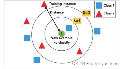
Q5. What is KNN Classifier ?

KNN means K-Nearest Neighbour Algorithm. It can be used for both classification and regression. KNN（K-最近邻）分类器是一种简单的机器学习算法，可以用于分类和回归任务。它被认为是最简单的机器学习算法之一，也称为懒惰学习算法。之所以称为懒惰学习，是因为它在训练阶段不会创建一个泛化的模型，而是将所有的工作推迟到测试阶段，在测试阶段进行实际的分类或回归任务。因此，测试阶段在时间和金钱上的成本都很高。KNN也被称为基于实例的学习或基于记忆的学习，因为它需要保留所有的训练数据。

It is the simplest machine learning algorithm. Also known as lazy learning (why? Because it does not create a generalized model during the time of training, so the testing phase is very important where it does the actual job. Hence Testing is very costly - in terms of time & money). Also called an instance- based or memory-based learning

In k-NN classification, the output is a class membership. An object is classified by a plurality vote of its neighbors, with the object being assigned to the class most common among its k nearest neighbors (k is a positive integer, typically small). If k = 1, then the object is assigned to the class of that single nearest neighbor.

KNN的工作原理如下：

1. 选择K的值：K是一个用户定义的常数，表示最近邻居的数量。
2. 计算距离：对于一个未分类的样本，计算它与训练集中每个样本之间的距离。常用的距离度量包括欧氏距离、曼哈顿距离等。
3. 找到最近的K个邻居：从训练集中选择距离最近的K个样本作为最近邻居。
4. 进行投票：对于分类问题，基于最近的K个邻居的类别进行多数投票来决定未分类样本的类别；对于回归问题，通常取最近的K个邻居的输出值的平均值作为预测结果。

KNN算法的优点包括简单、直观和易于实现，但它的缺点是对大数据集的计算和存储要求较高，且对于具有不同尺度的特征敏感，可能需要进行特征缩放。此外，选择合适的K值对算法的性能也非常关键。

在k-NN回归中，输出是对象的属性值，这个值是其k个最近邻居值的平均值。以下是几种常用的距离度量方法的简单解释：

1. 欧几里得距离（Euclidean Distance）：最常用的距离度量方法，可以被理解为两点间直线的长度。在二维空间中，就像我们使用直尺测量两点之间的距离。公式为：其中，x 和 y 是两个点，i 是维度数。

2. 曼哈顿距离（Manhattan Distance）：也称为城市街区距离，因为它像在规划有规则的城市街区中行走时，需要沿着街区边缘走的距离。公式为：^。

3. 闵可夫斯基距离（Minkowski Distance）：是欧几里得距离和曼哈顿距离的一般形式，公式为：^。其中，当 q=2 时，就是欧几里得距离；当 q=1 时，就是曼哈顿距离。

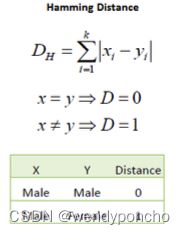
4. 汉明距离（Hamming Distance）: 对于连续变量，欧几里得距离、曼哈顿距离和闵可夫斯基距离是常用的距离度量方法。然而，在处理分类变量时，这些距离度量方法可能不再适用。

   汉明距离用于度量两个等长字符串之间的差异，即对应位置的字符不同的数量。在分类变量的上下文中，汉明距离可以被理解为两个观测值在分类属性上不一致特征的数量。例如，如果有两个观测值，它们在五个分类属性上的值分别为（A, B, C, D, E）和（A, B, X, D, Z），那么这两个观测值之间的汉明距离为2，因为有两个属性的值不匹配。

   汉明距离特别适用于处理只包含“是”或“否”、"0"或"1"这类二元特征的数据集，因为它简单地计算了两个观测值之间不一致的特征数。

   使用汉明距离时需要注意的一点是，它假设所有的属性同等重要。如果某些分类变量比其他变量更重要，可能需要考虑使用加权的距离度量方法，以便更准确地反映不同特征的重要性。

How to choose the value of K: K value is a hyperparameter which needs to choose during the time of model building

Also, a small number of neighbors are most flexible fit, which will have a low bias, but the high variance and a large number of neighbors will have a smoother decision boundary, which means lower variance but higher bias.

We should choose an odd number if the number of classes is even. It is said the most common values are to be 3 & 5.

Q6. What is Pipeline in sklearn ?

A pipeline is what chains several steps together, once the initial exploration is done. For example, some codes are meant to transform features — normalize numerically, or turn text into vectors, or fill up missing data, and they are transformers; other codes are meant to predict variables by fitting an algorithm,  such as random forest or support vector machine, they are estimators. Pipeline chains all these together, which can then be applied to training data in block.
Example of a pipeline that imputes data with the most frequent value of each column, and then fit a decision tree classifier.

From sklearn.pipeline import Pipeline
steps = [('imputation', Imputer(missing_values='NaN', strategy = 'most_frequent', axis=0)),
('clf', DecisionTreeClassifier())]
pipeline = Pipeline(steps)
clf = pipeline.fit(X_train,y_train)```

在sklearn（scikit-learn）中，管道（Pipeline）是一种工具，用于将多个数据处理步骤和模型训练步骤串联起来形成一个处理流程。这些步骤可以包括数据预处理（如归一化、文本向量化、缺失数据填充等），特征选择，以及使用算法进行模型的训练和预测等。每个步骤都是一个转换器（transformer）或一个估计器（estimator）。

使用管道的好处包括：

1. 简化代码：通过将数据预处理和模型训练步骤封装在一起，管道简化了机器学习工作流程的代码实现。
2. 避免数据泄露：在模型训练过程中，保证数据预处理步骤（如特征缩放、归一化）是在每次交叉验证的训练集上独立完成的，而不是在整个数据集上完成的，从而避免了数据泄露问题。
3. 方便的模型评估和参数调整：通过管道，可以将整个流程作为一个整体进行交叉验证和超参数调整，而不需要对每个步骤单独进行调整。

一个简单的管道示例可能包括以下几个步骤：

1. 使用StandardScaler对数值特征进行标准化。
2. 使用PCA进行特征降维。
3. 使用LogisticRegression进行分类。

Instead of fitting to one model, it can be looped over several models to find the best one.

classifiers = [ KNeighborsClassifier(5), RandomForestClassifier(), GradientBoostingClassifier()] for clf in classifiers:
steps = [('imputation', Imputer(missing_values='NaN', strategy = 'most_frequent', axis=0)),('clf', clf)]
pipeline = Pipeline(steps)

I also learned the pipeline itself can be used as an estimator and passed to cross-validation or grid search.

在sklearn中创建管道的代码如下：

from sklearn.model_selection import KFold
from sklearn.model_selection import cross_val_score
kfold = KFold(n_splits=10, random_state=seed)
results = cross_val_score(pipeline, X_train, y_train, cv=kfold)
print(results.mean())

在这个例子中，Pipeline对象pipeline将数据预处理和模型训练步骤封装在一起，使得从原始数据到最终预测的整个过程更加高效和一致。

Q7. What is Principal Component Analysis(PCA), and why we do?

主成分分析（PCA）的主要思想是降低由许多相互之间存在着轻度或重度相关的变量构成的数据集的维度，同时尽可能地保留数据集中存在的变异。这是通过将变量转换为一组新的变量来实现的，这组新变量被称为主成分（PCs），它们是正交的，并且按照顺序排列，使得保留在原始变量中的变异随着顺序的下降而减少。因此，第一个主成分保留了原始组成部分中存在的最大变异。主成分是协方差矩阵的特征向量，因此它们是正交的。

进行PCA的原因包括：

1. 降维：在包含大量特征的数据集中，不是所有特征都是有用的，PCA可以帮助识别最重要的特征。
2. 可视化：通过降维，PCA可以帮助我们将高维数据可视化为二维或三维图形，从而更容易地进行探索性数据分析。
3. 去除噪声：PCA通过保留最重要的成分，可以帮助去除数据中的噪声。
4. 优化算法性能：降维可以减少计算资源的需求，提高算法的运行效率。

使用sklearn中的管道进行数据预处理和模型训练的示例代码如下：

from sklearn.pipeline import Pipeline
from sklearn.impute import SimpleImputer
from sklearn.tree import DecisionTreeClassifier
from sklearn.model_selection import KFold
from sklearn.model_selection import cross_val_score

# 定义管道步骤
steps = [
    ('imputation', SimpleImputer(missing_values=np.nan, strategy='most_frequent')),
    ('clf', DecisionTreeClassifier())
]

# 创建管道
pipeline = Pipeline(steps)

# 使用k折交叉验证评估管道
kfold = KFold(n_splits=10, random_state=42)
results = cross_val_score(pipeline, X_train, y_train, cv=kfold)

print("交叉验证结果的平均值:", results.mean())

Q8. What is t-SNE? - 不熟悉

(t-SNE) t-Distributed Stochastic Neighbor Embedding is a non-linear dimensionality reduction algorithm used for exploring high-dimensional data. It maps multi-dimensional data to two or more dimensions suitable for human observation. With the help of the t-SNE algorithms, you may have to plot fewer exploratory data analysis plots next time you work with high dimensional data. t-SNE（t-分布随机邻域嵌入）是一种用于探索高维数据的非线性降维算法。它能将多维数据映射到两维或更多维，使其适合人类观察。t-SNE特别适合于数据可视化的任务，因为它能够在低维空间中保持高维数据点之间的局部结构，从而使得相似的数据点在降维后的空间中也保持相近。

t-SNE的关键特点包括：

• 非线性降维：与PCA等线性降维方法不同，t-SNE能够捕捉数据中的复杂非线性结构。
• 局部结构保留：t-SNE通过保留数据点之间的局部相似性来进行降维，这使得算法特别适用于揭示数据中的簇或群组。
• 参数选择：t-SNE算法中有几个关键参数，包括感知参数（perplexity）和学习率，这些参数的选择对最终的可视化结果有较大影响。

使用t-SNE进行高维数据可视化的步骤大致如下：

1. 选择合适的参数：感知参数通常设置在5到50之间，学习率通常设置在10到1000之间。参数的选择取决于数据的具体情况，可能需要尝试不同的值来获得最佳的可视化效果。
2. 运行t-SNE算法：使用t-SNE算法对高维数据进行降维处理，通常将数据降到二维或三维空间中。
3. 数据可视化：将降维后的数据绘制为散点图，观察数据点的分布，寻找可能的模式或簇。

t-SNE是一种强大的工具，特别适合于探索性数据分析和高维数据的可视化。通过使用t-SNE，你可以在处理高维数据时减少探索性数据分析所需绘制的图形数量，快速直观地识别数据中的模式和结构。

Q9. VIF(Variation Inflation Factor),Weight of Evidence & Information Value. Why and when to use?

方差膨胀因子（VIF，Variance Inflation Factor）是一种用来衡量多重共线性程度的指标。多重共线性是指模型中的一个或多个解释变量彼此高度相关的情况，这可能会导致回归模型的估计参数变得不准确或不稳定。

为什么以及何时使用VIF：

• 诊断多重共线性：VIF提供了一个指数，用来衡量由于共线性导致估计的回归系数的方差（估计标准差的平方）增大的程度。当VIF的值大于5时，通常认为存在多重共线性问题，需要进一步处理。
• 改善模型精度和稳定性：通过识别并处理具有高VIF值的变量，可以改善模型的精度和稳定性，使模型的预测更加可靠。

Variation Inflation Factor 理解VIF：

• 如果某个预测变量的VIF值为5，这意味着该预测变量的系数方差是如果该预测变量与其他预测变量不相关时的5倍。换句话说，如果预测变量的VIF值为5，这意味着该预测变量的系数标准误差是如果该预测变量与其他预测变量不相关时的2.23倍（√5 = 2.23）。

如何计算VIF：

• VIF的计算公式为：VIF = 1 / (1-R-Square of j-th variable) where R2 of jth variable is the coefficient of determination of the model that includes all independent variables except the jth predictor.

• Where R-Square of j-th variable is the multiple R2 for the regression of Xj on the other independent variables (a regression that does not involve the dependent variable Y).
  If VIF > 5, then there is a problem with multicollinearity.

处理高VIF值的方法：

• 移除变量：考虑从模型中移除具有高VIF值的变量，尤其是当这些变量在理论上不是非常重要时。
• 合并变量：如果可能，可以将相关的变量合并为一个变量。
• 使用岭回归（Ridge Regression）：岭回归可以处理多重共线性问题，通过引入正则化项减少系数的大小。

Understanding VIF

If the variance inflation factor of a predictor variable is 5 this means that variance for the coefficient of that predictor variable is 5 times as large as it would be if that predictor variable were uncorrelated with the other predictor variables.
In other words, if the variance inflation factor of a predictor variable is 5 this means that the standard

error for the coefficient of that predictor variable is 2.23 times (√5 = 2.23) as large as it would be if that predictor variable were uncorrelated with the other predictor variables.

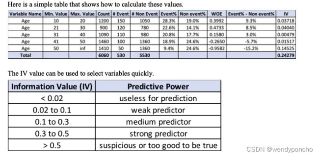
Weight of evidence (WOE) and information value (IV) are simple, yet powerful techniques to perform variable transformation and selection.

Q10: How to evaluate that data does not have any outliers ?

In statistics, outliers are data points that don’t belong to a certain population. It is an abnormal observation that lies far away from other values. An outlier is an observation that diverges from otherwise well- structured data.
Detection:

Method 1 — Standard Deviation: In statistics, If a data distribution is approximately normal, then about 68% of the data values lie within one standard deviation of the mean, and about 95% are within two standard deviations, and about 99.7% lie within three standard deviations.

Therefore, if you have any data point that is more than 3 times the standard deviation, then those points are very likely to be anomalous or outliers.

Method 2 — Boxplots: Box plots are a graphical depiction of numerical data through their quantiles. It is a very simple but effective way to visualize outliers. Think about the lower and upper whiskers as the boundaries of the data distribution. Any data points that show above or below the whiskers can be considered outliers or anomalous.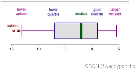

Method 3 - Violin Plots: Violin plots are similar to box plots, except that they also show the probability density of the data at different values, usually smoothed by a kernel density estimator. Typically a violin plot will include all the data that is in a box plot: a marker for the median of the data, a box or marker indicating the interquartile range, and possibly all sample points if the number of samples is not too high.

Method 4 - Scatter Plots: A scatter plot is a type of plot or mathematical diagram using Cartesian coordinates to display values for typically two variables for a set of data. The data are displayed as a collection of points, each having the value of one variable determining the position on the horizontal axis and the value of the other variable determining the position on the vertical axis.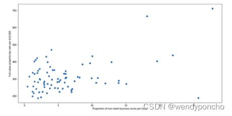

The points which are very far away from the general spread of data and have a very few neighbors are considered to be outliers.

Q11: What you do if there are outliers?

处理异常值（outliers）是数据预处理中的一个重要步骤，因为异常值可能会扭曲统计分析的结果，影响模型的性能。以下是一些常见的处理异常值的方法：

1. 删除异常值（Drop the Outliers）

如果异常值的数量不多，而且它们的存在对分析结果的影响很大，可以考虑直接删除这些异常值。这种方法简单直接，但要小心使用，因为删除数据可能会导致信息丢失。

2. 赋予新值（Assign a New Value）

如果异常值看起来是由数据录入错误或其他问题导致的，可以考虑对其进行修正或赋予一个合理的新值。这可以通过多种方式实现，如使用中位数、均值、或者基于其他变量的预测值来填充异常值。

3. 分组处理（Grouping and Separate Analysis）

如果异常值占比较小，但在数量上有很多，直接删除可能会损失重要的信息。在这种情况下，可以考虑将异常值分为一个单独的组，并对这个组进行单独的分析。这样做可以避免异常值对主要数据分析造成影响，同时又能够探索这些异常值背后可能存在的模式或原因。

其他方法：

• 变换数据：有时通过对数据进行变换（如对数变换、平方根变换等）可以减少异常值的影响。
• 使用鲁棒的统计方法：一些统计方法和模型对异常值不敏感，如中位数、IQR（四分位数间距）等。
• 离群值检测算法：使用专门的算法来检测和处理异常值，如箱型图、Z分数、DBSCAN等。

处理异常值时，重要的是先理解异常值的来源和性质，以及它们对分析或模型可能产生的影响。在删除或修正异常值之前，最好对数据进行彻底的探索性数据分析（EDA），并考虑到特定领域的知识和业务背景。

Q12: What are the encoding techniques you have applied with Examples ?

在许多实际的数据科学活动中，数据集会包含分类变量。这些变量通常以文本值的形式存储。由于机器学习基于数学方程，如果保持分类变量原样，会导致问题。考虑以下包含水果名称和它们重量的数据集为例，我们可以使用一些常见的编码技术来处理分类变量：

标签编码（Label Encoding）

在标签编码中，我们将每个类别映射到一个数字或标签。为类别选择的标签之间没有关系。因此，在编码后，那些有某些联系或彼此接近的类别会丢失这类信息。例如，如果有一个水果类别变量，包含“苹果”、“香蕉”和“橙子”，通过标签编码，它们可能被分别编码为1、2和3。这种方法简单直接，但不适用于模型中存在类别顺序或重要性的情况。

独热编码（One-Hot Encoding）

在这种方法中，我们将每个类别映射到一个包含1和0的向量，1表示特征的存在，0表示特征的不存在。向量的数量取决于我们想要保留的类别数量。对于高基数（许多唯一值）的特征，这种方法会产生大量的列，显著降低学习速度。继续上面的例子，通过独热编码，“苹果”、“香蕉”和“橙子”可能分别被编码为[1, 0, 0]、[0, 1, 0]和[0, 0, 1]。这种方法适用于没有顺序关系的类别特征，但会增加数据的维度。

Q13: Tradeoff between bias and variances, the relationship between them.

Whenever we discuss model prediction, it’s important to understand prediction errors (bias and variance). The prediction error for any machine learning algorithm can be broken down into three parts:

• Bias Error

• Variance Error

• Irreducible Error

The irreducible error cannot be reduced regardless of what algorithm is used. It is the error introduced from the chosen framing of the problem and may be caused by factors like unknown variables that influence the mapping of the input variables to the output variable.

Bias: Bias means that the model favors one result more than the others. Bias is the simplifying assumptions made by a model to make the target function easier to learn. The model with high bias pays very little attention to the training data and oversimplifies the model. It always leads to a high error in training and test data.

Variance: Variance is the amount that the estimate of the target function will change if different training data was used. The model with high variance pays a lot of attention to training data and does not generalize on the data which it hasn’t seen before. As a result, such models perform very well on training data but have high error rates on test data.

So, the end goal is to come up with a model that balances both Bias and Variance. This is called Bias Variance Trade-off. To build a good model, we need to find a good balance between bias and variance such that it minimizes the total error.

Q14: What is the difference between Type 1 and Type 2 error and severity of the error?

Type I Error

A Type I error is often referred to as a “false positive" and is the incorrect rejection of the true null hypothesis in favor of the alternative.
In the example above, the null hypothesis refers to the natural state of things or the absence of the tested effect or phenomenon, i.e., stating that the patient is HIV negative. The alternative hypothesis states that the patient is HIV positive. Many medical tests will have the disease they are testing for as the alternative hypothesis and the lack of that disease as the null hypothesis. A Type I error would thus occur when the patient doesn’t have the virus, but the test shows that they do. In other words, the test incorrectly rejects the true null hypothesis that the patient is HIV negative.

• 又称为“假阳性”（False Positive）。
• 发生在错误地拒绝了真实的零假设（即，实际上零假设是正确的，但测试结果错误地支持了备择假设）。
• 在HIV检测的例子中，如果患者实际上没有HIV病毒，但检测结果错误地显示他们感染了HIV病毒，这就是一个类型I错误。
• 类型I错误的严重性取决于具体情境。在某些情况下，如HIV检测，一个假阳性可能导致不必要的焦虑和进一步的检测，但最终可以通过进一步的测试来纠正。

Type II Error

A Type II error is the inverse of a Type I error and is the false acceptance of a null hypothesis that is not true, i.e., a false negative. A Type II error would entail the test telling the patient they are free of HIV when they are not.

Considering this HIV example, which error type do you think is more acceptable? In other words, would you rather have a test that was more prone to Type I or Types II error? With HIV, the momentary stress of a false positive is likely better than feeling relieved at a false negative and then failing to take steps to treat the disease. Pregnancy tests, blood tests, and any diagnostic tool that has serious consequences for the health of a patient are usually overly sensitive for this reason – they should err on the side of a false positive.

But in most fields of science, Type II errors are seen as less serious than Type I errors. With the Type II error, a chance to reject the null hypothesis was lost, and no conclusion is inferred from a non-rejected null. But the Type I error is more serious because you have wrongly rejected the null hypothesis and ultimately made a claim that is not true. In science, finding a phenomenon where there is none is more egregious than failing to find a phenomenon where there is.

• 又称为“假阴性”（False Negative）。
• 发生在错误地接受了不真实的零假设（即，实际上备择假设是正确的，但测试结果错误地支持了零假设）。
• 在HIV检测的例子中，如果患者实际上感染了HIV病毒，但检测结果错误地显示他们没有感染HIV病毒，这就是一个类型II错误。
• 类型II错误的严重性也取决于具体情况。在HIV检测的情况下，一个假阴性可能会导致患者错过及早治疗的机会，这可能比类型I错误的后果更加严重。

错误类型的选择

• 在不同的应用领域中，对类型I错误和类型II错误的容忍度不同。在医学检测（如HIV检测）中，人们可能更倾向于避免类型II错误，因为错过疾病的诊断可能导致严重的后果。
• 在大多数科学领域，类型I错误被认为比类型II错误更严重，因为错误地拒绝零假设可能导致错误的科学发现，这可能会误导后续的研究和政策制定。

总的来说，无论是类型I错误还是类型II错误，都需要根据研究的具体背景和对结果准确性的需求来综合考虑，并采取相应的统计方法和实验设计来尽可能地减少这些错误的发生。

Q15: What is binomial distribution and polynomial distribution?

Binomial Distribution: A binomial distribution can be thought of as simply the probability of a SUCCESS or FAILURE outcome in an experiment or survey that is repeated multiple times. The binomial is a type of distribution that has two possible outcomes (the prefix “bi” means two, or twice). For example, a coin toss has only two possible outcomes: heads or tails, and taking a test could have two possible outcomes: pass or fail.

二项分布（Binomial Distribution）

• 二项分布是一种离散概率分布，用来描述在固定次数的独立实验中，成功次数的概率分布，每次实验只有两种可能结果（成功或失败），并且每次实验成功的概率相同。
• 例如，抛掷硬币10次，正面朝上的次数就服从二项分布。在这个例子中，每次抛掷硬币正面朝上可以视为“成功”，硬币有两面，所以是两种结果的实验。
• 二项分布的概率质量函数（PMF）

Multimonial/Polynomial Distribution:Multi or Poly means many. In probability theory, the multinomial distribution is a generalization of the binomial distribution. For example, it models the probability of counts of each side for rolling a k-sided die n times. For n independent trials each of which leads to success for exactly one of k categories, with each category having a given fixed success probability, the multinomial distribution gives the probability of any particular combination of numbers of successes for the various categories.

多项分布（Multinomial/Polyomial Distribution）

• 多项分布是二项分布的推广，用于描述在固定次数的独立实验中，每种可能结果的次数的概率分布，每次实验有多于两种可能的结果，并且每种结果发生的概率固定。
• 例如，掷一个六面的骰子10次，各面朝上次数的分布就服从多项分布。在这个例子中，每次掷骰子有六种可能的结果。

Q16: What is the Mean Median Mode standard deviation for the sample and population?

Mean It is an important technique in statistics. Arithmetic Mean can also be called an average. It is the number of the quantity obtained by summing two or more numbers/variables and then dividing the sum by the number of numbers/variables.

Mode The mode is also one of the types for finding the average. A mode is a number that occurs most frequently in a group of numbers. Some series might not have any mode; some might have two modes, which is called a bimodal series.
In the study of statistics, the three most common ‘averages’ in statistics are mean, median, and mode.

Median is also a way of finding the average of a group of data points. It’s the middle number of a set of numbers. There are two possibilities, the data points can be an odd number group, or it can be an even number group.
If the group is odd, arrange the numbers in the group from smallest to largest. The median will be the one which is exactly sitting in the middle, with an equal number on either side of it. If the group is even, arrange the numbers in order and pick the two middle numbers and add them then divide by 2. It will be the median number of that set.

Standard Deviation (Sigma) Standard Deviation is a measure of how much your data is spread out in statistics.

Q17: What is Mean Absolute Error ?

What is Absolute Error? Absolute Error is the amount of error in your measurements. It is the difference between the measured value and the “true” value. For example, if a scale states 90 pounds, but you know your true weight is 89 pounds, then the scale has an absolute error of 90 lbs – 89 lbs = 1 lbs.

This can be caused by your scale, not measuring the exact amount you are trying to measure. For example, your scale may be accurate to the nearest pound. If you weigh 89.6 lbs, the scale may “round up” and give you 90 lbs. In this case the absolute error is 90 lbs – 89.6 lbs = .4 lbs.

Mean Absolute Error The Mean Absolute Error(MAE) is the average of all absolute errors. The formula is: mean absolute error

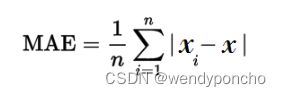
Where, n = the number of errors, Σ = summation symbol (which means “add them all up”), |xi – x| = the absolute errors. The formula may look a little daunting, but the steps are easy:
Find all of your absolute errors, xi – x. Add them all up. Divide by the number of errors. For example, if you had 10 measurements, divide by 10.

Q18: What is the difference between long data and wide data?

There are many different ways that you can present the same dataset to the world. Let's take a look at one of the most important and fundamental distinctions, whether a dataset is wide or long.
The difference between wide and long datasets boils down to whether we prefer to have more columns in our dataset or more rows.

Wide Data A dataset that emphasizes putting additional data about a single subject in columns is called a wide dataset because, as we add more columns, the dataset becomes wider.

Long Data Similarly, a dataset that emphasizes including additional data about a subject in rows is called a long dataset because, as we add more rows, the dataset becomes longer. It's important to point out that there's nothing inherently good or bad about wide or long data.
In the world of data wrangling, we sometimes need to make a long dataset wider, and we sometimes need to make a wide dataset longer. However, it is true that, as a general rule, data scientists who embrace the concept of tidy data usually prefer longer datasets over wider ones.

Q19: What are the data normalization method you have applied, and why?

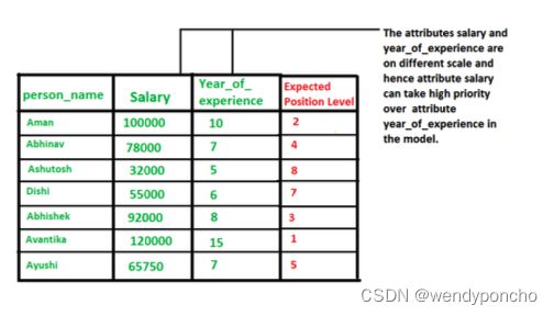
Normalization is a technique often applied as part of data preparation for machine learning. The goal of normalization is to change the values of numeric columns in the dataset to a common scale, without distorting differences in the ranges of values. For machine learning, every dataset does not require normalization. It is required only when features have different ranges. In simple words, when multiple attributes are there, but attributes have values on different scales, this may lead to poor data models while performing data mining operations. So they are normalized to bring all the attributes on the same scale, usually something between (0,1).

It is not always a good idea to normalize the data since we might lose information about maximum and minimum values. Sometimes it is a good idea to do so.

For example, ML algorithms such as Linear Regression or Support Vector Machines typically converge faster on normalized data. But on algorithms like K-means or K Nearest Neighbours, normalization could be a good choice or a bad depending on the use case since the distance between the points plays a key role here.

Types of Normalisation :

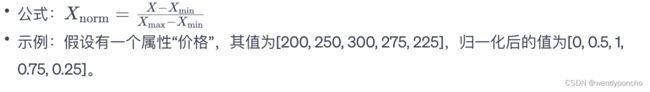
1. 最小-最大归一化（Min-Max Normalization）

这种方法通过将数据缩放到[0,1]区间来进行归一化。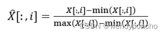

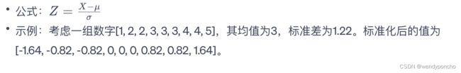
2. Z得分归一化（Z-Score Normalization）

这种方法基于原始数据的均值（μ）和标准差（σ）进行归一化，使得归一化后的数据具有均值为0和标准差为1的特性。

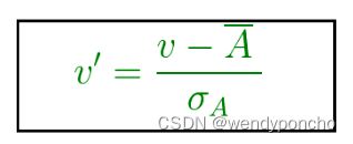
v’, v is new and old of each entry in data respectively. σA, A is the standard deviation and mean of A respectively standardization (or Z-score normalization) is that the features will be rescaled so that they’ll have the properties of a standard normal distribution with μ=0 and σ=1 where μ is the mean (average) and σ is the standard deviation from the mean; standard scores (also called z scores) of the samples are calculated as follows: z=(x−μ)/σ

3. 小数定标归一化（Decimal Scaling）

这种方法通过移动数据的小数点位置来进行归一化，小数点的移动位数取决于数据绝对值的最大值。

Q20: What is the difference between normalization and Standardization with example?

在机器学习中，特征缩放是一个重要的步骤，常用的方法包括归一化（Normalization）和标准化（Standardization）。

归一化（Normalization）

• 归一化通常指的是将数值缩放到[0, 1]的范围内。
• 归一化的目的是将不同尺度的特征转换到相同的尺度上，避免因为特征值范围的差异而对模型训练产生不良影响。

标准化（Standardization）

• 标准化通常指的是将数据缩放使其具有0的均值和1的标准差。
• 标准化的目的是将特征值转换为更接近正态分布的形式，这对于许多机器学习算法尤其是那些假设数据为正态分布的算法来说非常重要。

选择归一化还是标准化

• 归一化通常在需要将数值直接映射到特定范围时使用，特别是在神经网络中或者当数据不遵循高斯分布时。
• 标准化在数据遵循高斯分布或者算法（如支持向量机、线性回归、逻辑回归）假设数据遵循高斯分布时更为常见。

在实际应用中，归一化和标准化的选择取决于数据的特性和所选用的机器学习算法。有时，甚至可能结合使用归一化和标准化，以达到最佳的数据预处理效果。