Optional Lab: Feature Engineering and Polynomial Regression

Goals

In this lab you will explore feature engineering(特征工程) and polynomial regression(多项式回归)，使我们可以使用线性回归机制来拟合非常复杂甚至非线性的函数

Tools

You will utilize the function developed in previous labs as well as matplotlib and NumPy.

import numpy as np
import matplotlib.pyplot as plt
from lab_utils_multi import zscore_normalize_features, run_gradient_descent_feng
np.set_printoptions(precision=2)  # reduced display precision on numpy arrays

Feature Engineering and Polynomial Regression Overview

线性回归提供了一种建立以下形式的模型的方式
$$f_{\mathbf{w},b}=w_0{x}_0+w_1{x}_1+...+w_{n-1}{x}_{n-1}+b\text{\hspace{1em}(1)}$$
如果特征/数据是非线性的或是特征的组合该怎么办？例如，房价不倾向于与居住面积成线性关系but penalize very small or very large houses resulting in the curves shown in the graphic above，我们如何使用线性回归机制来拟合这条曲线？我们可以修改 (1) 中的参数 $\mathbf{w}$ 和 $\mathbf{b}$ 从而将方程“拟合”到训练数据，however no amount of adjusting of $\mathbf{w}$,$\mathbf{b}$ in (1) will实现对非线性曲线的拟合

Polynomial Features

上面我们考虑了一个数据是非线性的场景，让我们试着用我们目前学到的来拟合一条非线性曲线，从一个简单的二次方开始： $y=1+x^2$

You’re familiar with all the routines we’re using. 这些可以在文件lab_utils.py中查看，我们将使用np.c_[..] which is a NumPy routine to concatenate along the column boundary.

# create target data
x = np.arange(0, 20, 1)
y = 1 + x**2
X = x.reshape(-1, 1)

model_w,model_b = run_gradient_descent_feng(X,y,iterations=1000, alpha = 1e-2)

plt.scatter(x, y, marker='x', c='r', label="Actual Value"); plt.title("no feature engineering")
plt.plot(x,X@model_w + model_b, label="Predicted Value");  plt.xlabel("X"); plt.ylabel("y"); plt.legend(); plt.show()

输出如下

Iteration         0, Cost: 1.65756e+03
Iteration       100, Cost: 6.94549e+02
Iteration       200, Cost: 5.88475e+02
Iteration       300, Cost: 5.26414e+02
Iteration       400, Cost: 4.90103e+02
Iteration       500, Cost: 4.68858e+02
Iteration       600, Cost: 4.56428e+02
Iteration       700, Cost: 4.49155e+02
Iteration       800, Cost: 4.44900e+02
Iteration       900, Cost: 4.42411e+02
w,b found by gradient descent: w: [18.7], b: -52.0834

不出所料，并不是很合适，我们需要的是 $y=w_0{x}_0^2+b$ 或多项式特征，为此，可以修改input data to engineer the needed features
如果将原始数据 $x$ 替换为 $x$ 的平方，可以得到 $y=w_0{x}_0^2+b$ ，let’s try it

# create target data
x = np.arange(0, 20, 1)
y = 1 + x**2

# Engineer features 
X = x**2      #<-- added engineered feature

X = X.reshape(-1, 1)  #X should be a 2-D Matrix
model_w,model_b = run_gradient_descent_feng(X, y, iterations=10000, alpha = 1e-5)

plt.scatter(x, y, marker='x', c='r', label="Actual Value"); plt.title("Added x**2 feature")
plt.plot(x, np.dot(X,model_w) + model_b, label="Predicted Value"); plt.xlabel("x"); plt.ylabel("y"); plt.legend(); plt.show()

输出如下

Iteration         0, Cost: 7.32922e+03
Iteration      1000, Cost: 2.24844e-01
Iteration      2000, Cost: 2.22795e-01
Iteration         0, Cost: 7.32922e+03
Iteration      1000, Cost: 2.24844e-01
Iteration      2000, Cost: 2.22795e-01
Iteration      3000, Cost: 2.20764e-01
Iteration      4000, Cost: 2.18752e-01
Iteration      5000, Cost: 2.16758e-01
Iteration      3000, Cost: 2.20764e-01
Iteration      4000, Cost: 2.18752e-01
Iteration      5000, Cost: 2.16758e-01
Iteration      6000, Cost: 2.14782e-01
Iteration      7000, Cost: 2.12824e-01
Iteration      8000, Cost: 2.10884e-01
Iteration      6000, Cost: 2.14782e-01
Iteration      7000, Cost: 2.12824e-01
Iteration      8000, Cost: 2.10884e-01
Iteration      9000, Cost: 2.08962e-01
w,b found by gradient descent: w: [1.], b: 0.0490
Iteration      9000, Cost: 2.08962e-01
w,b found by gradient descent: w: [1.], b: 0.0490

近乎完美的拟合，注意 $\mathbf{w}$ 和 b 值在图像的正上方，梯度下降将 $\mathbf{w}$ 和 b 的初始值修改为 (1.0,0.049) 或者模型 $y=1\ast x_0^2+0.049$，与我们的目标 $y=1\ast x_0^2+1$ 非常接近，如果运行时间更长，会更加符合

Selecting Features

通过上面，我们知道 $x^2$ 项是必须的
需要哪些特征并不是显而易见的，我们可以通过尝试添加各种潜在的特征来找到最有用的，比如尝试： $y=w_0{x}_0+w_1{x}_1^2+w_2{x}_2^3+b$
运行以下代码

# create target data
x = np.arange(0, 20, 1)
y = x**2

# engineer features .
X = np.c_[x, x**2, x**3]   #<-- added engineered feature

model_w,model_b = run_gradient_descent_feng(X, y, iterations=10000, alpha=1e-7)

plt.scatter(x, y, marker='x', c='r', label="Actual Value"); plt.title("x, x**2, x**3 features")
plt.plot(x, X@model_w + model_b, label="Predicted Value"); plt.xlabel("x"); plt.ylabel("y"); plt.legend(); plt.show()

输出如下

Iteration         0, Cost: 1.14029e+03
Iteration      1000, Cost: 3.28539e+02
Iteration      2000, Cost: 2.80443e+02
Iteration         0, Cost: 1.14029e+03
Iteration      1000, Cost: 3.28539e+02
Iteration      2000, Cost: 2.80443e+02
Iteration      3000, Cost: 2.39389e+02
Iteration      4000, Cost: 2.04344e+02
Iteration      5000, Cost: 1.74430e+02
Iteration      3000, Cost: 2.39389e+02
Iteration      4000, Cost: 2.04344e+02
Iteration      5000, Cost: 1.74430e+02
Iteration      6000, Cost: 1.48896e+02
Iteration      7000, Cost: 1.27100e+02
Iteration      8000, Cost: 1.08495e+02
Iteration      6000, Cost: 1.48896e+02
Iteration      7000, Cost: 1.27100e+02
Iteration      8000, Cost: 1.08495e+02
Iteration      9000, Cost: 9.26132e+01
w,b found by gradient descent: w: [0.08 0.54 0.03], b: 0.0106
Iteration      9000, Cost: 9.26132e+01
w,b found by gradient descent: w: [0.08 0.54 0.03], b: 0.0106

注意 $\mathbf{w}$ 的值为[0.08 0.54 0.03]，b 的值为 0.0106，这意味着拟合/训练后的模型为：
$$0.08x+0.54x^2+0.03x^3+0.0106$$
梯度下降强调了最适合 $x^2$ 的数据是通过增加 $w_1$ 项（相比其他项来说）实现的，如果要运行很长时间，它将持续减少其他项的影响
因为梯度下降是通过强调其他相关参数来选择“正确”的特征的

让我们回顾一下这个想法：

• 首先，这些特征被重新放缩，以便相互比较
• 较小的权重值意味着不太重要/正确的特征，在极端情况下，当权重变成0或者非常接近0时，相关的特征在模型拟合数据中是有用的
• 以上，在拟合后，与 $x^2$ 这个特征相关的权重比 $x$ 或 $x^3$ 大得多，因为它在拟合数据中是最useful的

An Alternate View

多项式特征是根据它们与目标数据的匹配程度来选择的
另外，一旦我们创建了新的功能，需要注意我们仍在使用线性回归，考虑到这一点，最佳特征将是相对于目标的线性特征
通过一个例子来理解这一点

# create target data
x = np.arange(0, 20, 1)
y = x**2

# engineer features .
X = np.c_[x, x**2, x**3]   #<-- added engineered feature
X_features = ['x','x^2','x^3']

fig,ax=plt.subplots(1, 3, figsize=(12, 3), sharey=True)
for i in range(len(ax)):
    ax[i].scatter(X[:,i],y)
    ax[i].set_xlabel(X_features[i])
ax[0].set_ylabel("y")
plt.show()

通过上图可以看出，很明显根据目标值 $y$ 映射的特征 $x^2$ 是线性的，线性回归可以很容易地使用该特征生成模型。

Scaling features

如上一个lab所述，如果数据集有明显不同尺度的特征，则应实行特征放缩来加快梯度下降
在上面的例子中， $x$ 、$x^2$ 和 $x^3$ 明显具有非常不同的尺度，让我们对其运用归一化

# create target data
x = np.arange(0,20,1)
X = np.c_[x, x**2, x**3]
print(f"Peak to Peak range by column in Raw        X:{np.ptp(X,axis=0)}")

# add mean_normalization 
X = zscore_normalize_features(X)     
print(f"Peak to Peak range by column in Normalized X:{np.ptp(X,axis=0)}")

输出如下

Peak to Peak range by column in Raw        X:[  19  361 6859]
Peak to Peak range by column in Normalized X:[3.3  3.18 3.28]

现在我们可以使用更激进的alpha值重新尝试

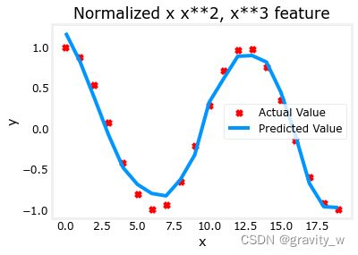
x = np.arange(0,20,1)
y = x**2

X = np.c_[x, x**2, x**3]
X = zscore_normalize_features(X) 

model_w, model_b = run_gradient_descent_feng(X, y, iterations=100000, alpha=1e-1)

plt.scatter(x, y, marker='x', c='r', label="Actual Value"); plt.title("Normalized x x**2, x**3 feature")
plt.plot(x,X@model_w + model_b, label="Predicted Value"); plt.xlabel("x"); plt.ylabel("y"); plt.legend(); plt.show()

输出如下

Iteration         0, Cost: 9.42147e+03
Iteration         0, Cost: 9.42147e+03
Iteration     10000, Cost: 3.90938e-01
Iteration     10000, Cost: 3.90938e-01
Iteration     20000, Cost: 2.78389e-02
Iteration     20000, Cost: 2.78389e-02
Iteration     30000, Cost: 1.98242e-03
Iteration     30000, Cost: 1.98242e-03
Iteration     40000, Cost: 1.41169e-04
Iteration     40000, Cost: 1.41169e-04
Iteration     50000, Cost: 1.00527e-05
Iteration     50000, Cost: 1.00527e-05
Iteration     60000, Cost: 7.15855e-07
Iteration     60000, Cost: 7.15855e-07
Iteration     70000, Cost: 5.09763e-08
Iteration     70000, Cost: 5.09763e-08
Iteration     80000, Cost: 3.63004e-09
Iteration     80000, Cost: 3.63004e-09
Iteration     90000, Cost: 2.58497e-10
Iteration     90000, Cost: 2.58497e-10
w,b found by gradient descent: w: [5.27e-05 1.13e+02 8.43e-05], b: 123.5000

特征缩放使其收敛得更快
再次注意 $\mathbf{w}$ 的值， $w_1$ 项即表明 $x^2$ 项是最受重视的，梯度下降几乎消除了 $x^3$ 项

Complex Functions

使用特征工程，即使非常复杂的函数也可以建模

x = np.arange(0,20,1)
y = np.cos(x/2)

X = np.c_[x, x**2, x**3,x**4, x**5, x**6, x**7, x**8, x**9, x**10, x**11, x**12, x**13]
X = zscore_normalize_features(X) 

model_w,model_b = run_gradient_descent_feng(X, y, iterations=1000000, alpha = 1e-1)

plt.scatter(x, y, marker='x', c='r', label="Actual Value"); plt.title("Normalized x x**2, x**3 feature")
plt.plot(x,X@model_w + model_b, label="Predicted Value"); plt.xlabel("x"); plt.ylabel("y"); plt.legend(); plt.show()

输出如下

Iteration         0, Cost: 2.24887e-01
Iteration         0, Cost: 2.24887e-01
Iteration    100000, Cost: 2.31061e-02
Iteration    100000, Cost: 2.31061e-02
Iteration    200000, Cost: 1.83619e-02
Iteration    200000, Cost: 1.83619e-02
Iteration    300000, Cost: 1.47950e-02
Iteration    300000, Cost: 1.47950e-02
Iteration    400000, Cost: 1.21114e-02
Iteration    400000, Cost: 1.21114e-02
Iteration    500000, Cost: 1.00914e-02
Iteration    500000, Cost: 1.00914e-02
Iteration    600000, Cost: 8.57025e-03
Iteration    600000, Cost: 8.57025e-03
Iteration    700000, Cost: 7.42385e-03
Iteration    700000, Cost: 7.42385e-03
Iteration    800000, Cost: 6.55908e-03
Iteration    800000, Cost: 6.55908e-03
Iteration    900000, Cost: 5.90594e-03
Iteration    900000, Cost: 5.90594e-03
w,b found by gradient descent: w: [-1.61e+00 -1.01e+01  3.00e+01 -6.92e-01 -2.37e+01 -1.51e+01  2.09e+01
 -2.29e-03 -4.69e-03  5.51e-02  1.07e-01 -2.53e-02  6.49e-02], b: -0.0073

Congratulations!

In this lab you:

• 学习了线性回归如何使用特征工程对复杂甚至高度非线性的函数进行建模
• 认识到在进行特征工程时使用特征放缩很重要