图神经网络预训练 (4) - 节点属性预测 Attribute Prediction + 监督学习 代码
我们继续剖析Strategies for Pre-training Graph Neural Networks一文。
上一文中介绍了子结构预测的预训练方法(Context Prediction)。对于一个多层的深度学习模型,在分子图上训练主模型,在子图上训练层数较少的子模型,限制(损失是)主模型上与子模型的嵌入向量相似,保证子结构环境相似的节点在随着模型的层数增加时仍能保持相似的嵌入向量,意味着化学环境相似的结构具有相似的嵌入向量,即模型学会了分子图的子结构。由此,该多层深度学习模型具有更好的泛化能力。
接下来,介绍另一种节点层面的预训练方法,节点属性预测的预训练方法(Attribute Prediction)及其随后的监督学习部分。 代码下载,请见文末。
一、Attribute prediction预训练介绍
属性掩码的示意图如下:
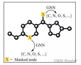
主要思路是:希望深度模型根据不同节点类型给出不同的节点嵌入向量(表示),即模型能学习到节点信息。
这就避免了:模型为了完成某一图层面的任务,完全不考虑节点之间差别,让性质完全不同的两个节点都表示成相似的向量,在另外一个图层面的任务上,该训练好模型,实际上是没有意义的,甚至起反效果。更不要提,在任务过程中,节点嵌入向量的有效性、重要性、解释性等。
具体流程:
(1)首先,将所有分子由SMILES转化成图,获得每个节点的特征和边的特征,包括,原子的类型和边的类型,同时随机选择一些节点及其相邻的边进行mask,属性值都归置为0,这些被mask的节点和边称之为mask节点/边;
(2)然后,通过一个图神经网络模型model,例如GAT,输入的分子每一个节点的属性嵌入embeding,生成每一个节点的特征,特征向量维度为:embeding_dim;
(3)将mask节点/边的特征,输入到一个简单的线性层linear_pred_node_model,linear_pred_edge_model分别去预测被掩盖节点、边的类型。
(4)由于线性层linear_pred_node_model非常简单,所以模型训练的时候,关于节点类型的预测的损失,都是来自于深度学习模型本身,使深度学习模型要对不同类型的节点输出不同的嵌入向量。
这样子模型就学会了节点层面上表征,具有更好的泛化能力。
损失函数:
linear_pred_node_model,linear_pred_edge_model预测的节点和边的类型与真实节点/边的类型的交叉熵
难点:
在由随机mask的情况下,在批次中,知道哪些些原子被mask,哪些边被mask,同时记录他们的原来的真实的类型。原来真实的类型作为模型的标签,用于计算损失。
注意:
图神经网络模型model可以是GAT,也可以是Transformer等其他模型
源代码中有很多其他的数据集,例如BBBP等,为了简单起见,这里仅仅使用zinc数据集。
由于,attribute prediction与context prediction有较多的模块可以共用,都在context prediction中已经介绍过了。这里直接挑重点来介绍。
二、数据预处理
使用MoleculeDataset类加载zinc数据集,每一个分子都生成PYG的Data类型,组成Dataset,并使用MaskAtom类对每一个分子的Data进行掩码转化。掩码转化指的是,掩盖部分的节点和相应边的特征,指定为新的类型,并记录原来真实的类型的过程。
dataset = MoleculeDataset(root="zinc_standard_agent", dataset='zinc_standard_agent',
                          transform = MaskAtom(num_atom_type = 119,
                                        num_edge_type = 4, mask_rate = 0.2,
                                        mask_edge=True))
注意,zinc数据集名称为zinc_standard_agent,保存在dataset/zinc_standard_agent/raw目录下。根据MoleculeDataset的要求,zinc数据集为压缩格式(.csv.gz)。运行完以后,会自动生成processed目录及其内容。再次运行上述部分时,会自动跳过,而直接调取*.pt文件。这一点要注意,如果你是直接从context prediction部分的dataset直接迁移过来,要删除*.pt文件,要不会报错的。dataset文件目录如下:

关于MaskAtom类要注意,比较关键,类似于context prediction中ExtractSubstructureContextPair类,不同的是,MaskAtom类是对于一个分子图,随机的掩盖部分的节点及其相连接的边,且记录真实节点和边的属性。属性主要是类别。
主要体现在对边和节点的处理上。对mask的节点和边:
for atom_idx in masked_atom_indices:
            mask_node_labels_list.append(data.x[atom_idx].view(1, -1))
        data.mask_node_label = torch.cat(mask_node_labels_list, dim=0) # 被mask节点的特征,即标签
        data.masked_atom_indices = torch.tensor(masked_atom_indices) # 被mask的节点序号
for bond_idx in connected_edge_indices:
                    data.edge_attr[bond_idx] = torch.tensor(
                        [self.num_edge_type, 0]) # 被mask边的特征修改成特定类型

                data.connected_edge_indices = torch.tensor(
                    connected_edge_indices[::2]) #被mask边的序号
MaskAtom类代码如下。注意我们将masking的节点和边,算作是另一种类别,而不是简单的所有特征置0。
class MaskAtom:
    def __init__(self, num_atom_type, num_edge_type, mask_rate, mask_edge=True):
        """
        :param num_atom_type: 原子类型个数
        :param num_edge_type: 边类型个数
        :param mask_rate: % of atoms to be masked 随机mask的比例
        :param mask_edge: If True, also mask the edges that connect to the 是否mask边
        masked atoms
        """
        self.num_atom_type = num_atom_type
        self.num_edge_type = num_edge_type
        self.mask_rate = mask_rate
        self.mask_edge = mask_edge

    def __call__(self, data, masked_atom_indices=None):
        """
        生成的是图层面的属性
        data.mask_node_idx 被mask的节点序号
        data.mask_node_label 被mask节点的特征,即标签
        data.mask_edge_idx 被mask边,与mask节点相连
        data.mask_edge_label 被mask边的特征
        """

        if masked_atom_indices == None:
            num_atoms = data.x.size()[0]
            sample_size = int(num_atoms * self.mask_rate + 1)
            masked_atom_indices = random.sample(range(num_atoms), sample_size) #随机抽取mask节点的序号
        mask_node_labels_list = []
        for atom_idx in masked_atom_indices:
            mask_node_labels_list.append(data.x[atom_idx].view(1, -1))
        data.mask_node_label = torch.cat(mask_node_labels_list, dim=0) # 被mask节点的特征,即标签
        data.masked_atom_indices = torch.tensor(masked_atom_indices) # 被mask的节点序号

        for atom_idx in masked_atom_indices:
            data.x[atom_idx] = torch.tensor([self.num_atom_type, 0]) #把mask节点的特征改为特定类型

        if self.mask_edge:
            connected_edge_indices = []
            for bond_idx, (u, v) in enumerate(data.edge_index.cpu().numpy().T):
                for atom_idx in masked_atom_indices:
                    if atom_idx in set((u, v)) and \
                        bond_idx not in connected_edge_indices:
                        connected_edge_indices.append(bond_idx) #记录与mask节点相邻的边

            if len(connected_edge_indices) > 0:
                mask_edge_labels_list = []
                for bond_idx in connected_edge_indices[::2]:
                    mask_edge_labels_list.append(
                        data.edge_attr[bond_idx].view(1, -1))

                data.mask_edge_label = torch.cat(mask_edge_labels_list, dim=0) #被mask边的特征/标签
                for bond_idx in connected_edge_indices:
                    data.edge_attr[bond_idx] = torch.tensor(
                        [self.num_edge_type, 0]) # 被mask边的特征修改成特定类型

                data.connected_edge_indices = torch.tensor(
                    connected_edge_indices[::2]) #被mask边的序号
            else:
                #如果没有mask的边,例如mask的节点是单节点,没有边就会出现这个情况
                data.mask_edge_label = torch.empty((0, 2)).to(torch.int64)
                data.connected_edge_indices = torch.tensor(
                    connected_edge_indices).to(torch.int64)
        return data

    def __repr__(self):
        return '{}(num_atom_type={}, num_edge_type={}, mask_rate={}, mask_edge={})'.format(
            self.__class__.__name__, self.num_atom_type, self.num_edge_type,
            self.mask_rate, self.mask_edge)
三、数据加载器
生词批次数据的难点在于,分子图中的mask_edge_label、mask_node_label两个标签,以及标签的位置索引masked_atom_indices和connected_edge_indices。
特别是后面两个标签位置索引。每个分子,被掩盖的原子和边数量不同,所以长度不一。然后,两个标签位置索引是数字,当分子图组成批次以后,原子的坐标被从新编码,所以原来的两个标签位置索引需要重新标记。
所以,需要专门有一个类,来处理。
loader = DataLoaderMasking(
    dataset, batch_size=64,
    shuffle=True, num_workers = 6) #加载数据集成dataloader,带批次
这里用的是DataLoaderMasking继承于torch.utils.data.DataLoader,如下:
class DataLoaderMasking(torch.utils.data.DataLoader):
    """
    将PYG的数据类型的一个个分子组装成dataloader,生成批次数据,
    主要利用BatchMasking进行
    """
    def __init__(self, dataset, batch_size=1, shuffle=True, **kwargs):
        super(DataLoaderMasking, self).__init__(
            dataset,
            batch_size,
            shuffle,
            collate_fn = lambda data_list: BatchMasking.from_data_list(data_list),
            **kwargs)
在DataLoaderMasking中,使用BatchMasking函数/类,实现对pyg分子图(小图)组成的list,加载成为批次(大图)。重点在于,于索引相关的特征,都要加上cumsum_node 或cumsum_edge 累计数值。如果是,与索引无关的,则不需要,直接叠加即可。其实就是为了处理:'edge_index', 'face', 'masked_atom_indices', 'connected_edge_indices'几个与索引相关的特征。如下:
class BatchMasking(Data):

    def __init__(self, batch=None, **kwargs):
        super(BatchMasking, self).__init__(**kwargs)
        self.batch = batch

    @staticmethod
    def from_data_list(data_list):

        keys = [set(data.keys) for data in data_list]
        keys = list(set.union(*keys)) #每一张图的属性
        assert 'batch' not in keys

        batch = BatchMasking()

        for key in keys:
            batch[key] = []
        #记录批次中每一个节点所属于的哪一个分子,[1,1,1,1,2,2,2,2,2,3,3,3,3,3]
        #有4个节点属于1号分子,位置在1~4,有5个节点属于2号分子,位置在5~9.
        #相当于节点的位置索引
        batch.batch = []
        #batch是一个Data类,用于保存批次中所有的数据

        cumsum_node = 0
        cumsum_edge = 0

        for i, data in enumerate(data_list):
            num_nodes = data.num_nodes #分子的节点数
            batch.batch.append(torch.full((num_nodes, ),
                                          i, dtype=torch.long)) #添加节点索引,例如:5号分子有3个节点:[5,5,5]
            for key in data.keys: #分子的所有特征
                item = data[key] #特征
                if key in ['edge_index', 'masked_atom_indices']: #与节点序号相关的特征都要累加节点的序号
                    item = item + cumsum_node
                elif key  == 'connected_edge_indices': #被mask边的序号也要累加,累加的是边的序号
                    item = item + cumsum_edge
                batch[key].append(item) #分子特征添加到批次中

            cumsum_node += num_nodes
            cumsum_edge += data.edge_index.shape[1]

        #把每一个key的特征组合在batch里面
        for key in keys:
            batch[key] = torch.cat(
                batch[key],
                dim=data_list[0].__cat_dim__(key, batch[key][0])) #返回创建小批量时将连接属性键的值的维度
        batch.batch = torch.cat(batch.batch, dim=-1)
        return batch.contiguous() #确保所有属性连续的内存布局

    def cumsum(self, key, item):
        return key in ['edge_index', 'face', 'masked_atom_indices', 'connected_edge_indices']

    @property
    def num_graphs(self):
        """Returns the number of graphs in the batch."""
        return self.batch[-1].item() + 1
四、模型
三个模型,model进行节点和节点层面的特征、linear_pred_atoms根据mask节点的特征预测mask节点原来的类型,linear_pred_bonds根据组成mask边的节点进行预测边的类型。
4.1 model
model我们还是用的文章中的GIN模型,让其输出一个256维的节点的嵌入向量。
model = GNN(7,256)关于model模型,可以替换成任何一个模型,例如GAT,transformer等。关于num_bond_type,是与MoleculeDataset中的num_edge_type等价的,MoleculeDataset已经设定为5种,里面包含:0~3是正常的键类型,5是mask类型,4是self-loop类型,所以,里面设定self-loop的键的类型为4。原来有119种原子,加上masking的类别那么就是120种。
class GINConv(MessagePassing):
    """
    文献中的GIN模型
    """
    def __init__(self, emb_dim, num_bond_type=5, num_bond_direction=3, aggr = "add"):
        super(GINConv, self).__init__(aggr = "add")
        #multi-layer perceptron
        self.mlp = torch.nn.Sequential(torch.nn.Linear(emb_dim, 2*emb_dim), torch.nn.ReLU(), torch.nn.Linear(2*emb_dim, emb_dim))
        self.edge_embedding1 = torch.nn.Embedding(num_bond_type, emb_dim)
        self.edge_embedding2 = torch.nn.Embedding(num_bond_direction, emb_dim)

        torch.nn.init.xavier_uniform_(self.edge_embedding1.weight.data)
        torch.nn.init.xavier_uniform_(self.edge_embedding2.weight.data)
        self.aggr = aggr

    def forward(self, x, edge_index, edge_attr):
        #add self loops in the edge space
        edge_index = add_self_loops(edge_index, num_nodes = x.size(0))[0]
        edge_index = edge_index.long()

        #add features corresponding to self-loop edges.
        self_loop_attr = torch.zeros(x.size(0), 2)
        self_loop_attr[:,0] = 4 #bond type for self-loop edge
        self_loop_attr = self_loop_attr.to(edge_attr.device).to(edge_attr.dtype)
        edge_attr = torch.cat((edge_attr, self_loop_attr), dim = 0)
        edge_embeddings = self.edge_embedding1(edge_attr[:,0]) + self.edge_embedding2(edge_attr[:,1])
        return self.propagate(edge_index=edge_index, x=x, edge_attr=edge_embeddings)

    def message(self, x_j, edge_attr):
        return x_j + edge_attr

    def update(self, aggr_out):
        return self.mlp(aggr_out)
class GNN(torch.nn.Module):

    def __init__(self, num_layer, emb_dim, num_atom_type=120, num_chirality_tag=4, JK = "last", drop_ratio = 0.5):
        super(GNN, self).__init__()
        self.num_layer = num_layer
        self.drop_ratio = drop_ratio
        self.JK = JK

        if self.num_layer < 2:
            raise ValueError("Number of GNN layers must be greater than 1.")

        self.x_embedding1 = torch.nn.Embedding(num_atom_type, emb_dim)
        self.x_embedding2 = torch.nn.Embedding(num_chirality_tag, emb_dim)

        torch.nn.init.xavier_uniform_(self.x_embedding1.weight.data)
        torch.nn.init.xavier_uniform_(self.x_embedding2.weight.data)

        self.gnns = torch.nn.ModuleList()
        for layer in range(num_layer):
            self.gnns.append(GINConv(emb_dim, aggr = "add"))

        self.batch_norms = torch.nn.ModuleList()
        for layer in range(num_layer):
            self.batch_norms.append(torch.nn.BatchNorm1d(emb_dim))

    def forward(self, *argv):
        if len(argv) == 3:
            x, edge_index, edge_attr = argv[0], argv[1], argv[2]
        elif len(argv) == 1:
            data = argv[0]
            x, edge_index, edge_attr = data.x, data.edge_index, data.edge_attr
        else:
            raise ValueError("unmatched number of arguments.")

        x = self.x_embedding1(x[:,0]) + self.x_embedding2(x[:,1])

        h_list = [x]
        for layer in range(self.num_layer):
            h = self.gnns[layer](h_list[layer], edge_index, edge_attr)
            h = self.batch_norms[layer](h)
            #h = F.dropout(F.relu(h), self.drop_ratio, training = self.training)
            if layer == self.num_layer - 1:
                #remove relu for the last layer
                h = F.dropout(h, self.drop_ratio, training = self.training)
            else:
                h = F.dropout(F.relu(h), self.drop_ratio, training = self.training)
            h_list.append(h)

        if self.JK == "concat":
            node_representation = torch.cat(h_list, dim = 1)
        elif self.JK == "last":
            node_representation = h_list[-1]
        elif self.JK == "max":
            h_list = [h.unsqueeze_(0) for h in h_list]
            node_representation = torch.max(torch.cat(h_list, dim = 0), dim = 0)[0]
        elif self.JK == "sum":
            h_list = [h.unsqueeze_(0) for h in h_list]
            node_representation = torch.sum(torch.cat(h_list, dim = 0), dim = 0)[0]

        return node_representation
4.2 linear_pred_atoms
根据节点的256维嵌入向量预测节点的原子类别,使用简单的线性层。
linear_pred_atoms = torch.nn.Linear(256, 119) #预测原子属性
linear_pred_atoms = linear_pred_atoms.to(device)
4.3 linear_pred_bonds
根据边的256维嵌入向量预测边的类别,使用简单的线性层。
linear_pred_bonds = torch.nn.Linear(256, 4).to(device) #预测边属性
linear_pred_bonds = linear_pred_bonds.to(device)
需要再次说明的是,linear_pred_atoms和linear_pred_bonds预测节点和边的类别,我们都是用非常简单的单层线性层,是为了将整个网络的损失,都集中在主模型model上,逼迫model在输出节点和边的嵌入时,不同类型节点和边的嵌入向量不同。
五、训练过程
训练过程的代码与之前的context prediction很类似。也有不一样的地方,主要是:损失函数是交叉熵,因为我们要预测节点和边的类别。
训练过程代码如下:
model = GNN(7,256)
model = model.to(device)
linear_pred_atoms = torch.nn.Linear(256, 119) #预测原子属性
linear_pred_atoms = linear_pred_atoms.to(device)

linear_pred_bonds = torch.nn.Linear(256, 4).to(device) #预测边属性
linear_pred_bonds = linear_pred_bonds.to(device)

#优化器
optimizer_model = optim.Adam(model.parameters(), lr=0.001,  weight_decay=1e-5)
optimizer_linear_pred_atoms = optim.Adam(linear_pred_atoms.parameters(), lr=0.001, weight_decay=1e-5)
optimizer_linear_pred_bonds = optim.Adam(linear_pred_bonds.parameters(), lr=0.001, weight_decay=1e-5)

epochs = 100
criterion = torch.nn.CrossEntropyLoss()

log_loss = []
log_acc_node = []
log_acc_edge = []

for epoch in range(epochs):
    model.train()
    linear_pred_atoms.train()
    linear_pred_bonds.train()

    loss_accum = 0
    acc_node_accum = 0
    acc_edge_accum = 0

    for step, batch in enumerate(tqdm(loader, desc='Iteration')):
        batch = batch.to(device)
        # model输出每一个节点的嵌入向量
        node_pre = model(batch)

        # linear_pred_atoms预测掩码节点属性
        pred_node = linear_pred_atoms(node_pre[batch.masked_atom_indices])
        # 节点损失
        loss = criterion(pred_node.double(), batch.mask_node_label[:, 0])  # 根据原子类型判断损失,这里原子的类型太多了!!
        # 原子类型预测精度
        node_acc = compute_accuracy(pred_node, batch.mask_node_label[:, 0])
        # 精度累加
        acc_node_accum = acc_node_accum + node_acc
        # 边预测损失,用mask边相关的节点的特征来预测边的类型
        mask_edge_index = batch.edge_index[:,
                          batch.connected_edge_indices]  # 被mask边的edge_index([1,2,3], [3,1,2])
        edge_rep = node_pre[mask_edge_index[0]] + node_pre[mask_edge_index[1]]
        pred_edge = linear_pred_bonds(edge_rep)  # 预测边的类型
        # 预测边的损失
        loss += criterion(pred_edge, batch.mask_edge_label[:, 0])
        optimizer_model.zero_grad()
        optimizer_linear_pred_atoms.zero_grad()
        optimizer_linear_pred_bonds.zero_grad()
        loss.backward()
        optimizer_model.step()
        optimizer_linear_pred_atoms.step()
        optimizer_linear_pred_bonds.step()
        loss_accum = loss_accum + loss.cpu().item()
        acc_edge = compute_accuracy(pred_edge, batch.mask_edge_label[:, 0])  # 预测边准确性
        # 精度累加
        acc_edge_accum += acc_edge
        # 记录批次损失和指标
    log_loss.append(loss_accum / (step + 1))
    log_acc_edge.append(acc_edge_accum / (step + 1))
    log_acc_node.append(acc_node_accum / (step + 1))
    # 保存损失和指标
    np.save("log_loss.npy", log_loss)
    np.save("log_acc_edge.npy", log_acc_edge)
    np.save("log_acc_node.npy", log_acc_node)

    print('Epoch:{},loss:{}, acc_node:{}, acc_edge:{}'.format(
        epoch, loss_accum / (step + 1), acc_node_accum / (step + 1), acc_edge_accum / (step + 1)))
    # 保存模型,由于模型训练时长很长,所以每次都要保存一下
    torch.save(model.state_dict(), "Net_GIN_para.pth")
    torch.save(model, "Net_GIN.pth")
    torch.save(linear_pred_atoms, 'linear_pred_atoms.pth')
    torch.save(linear_pred_bonds, 'linear_pred_bonds.pth')
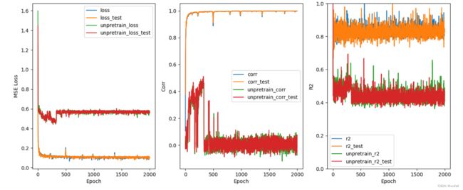
训练过程损失与精度曲线:

一个有趣的结果,边的特征训练结果比较好,种类准确率达到了98%,为节点的种类预测仅停留在92%以下。这很有可能是与节点的种类过多有关系的。因为节点种类有119种,而好多个种类其实并不会出现在数据集种的,例如什么镧系原子,自然结果准确率不高了。
再到过头一想,context prediction的准确率最后停留在80%左右,其实也不是很高。这很有可能是输入模型特征的问题。简单的通过添加深度学习模型的深度(层数)其实并不会有很大的改变,哪怕是全新的更有解释力的深度学习模型,例如transformer,效果估计也不会很好。也许,输入模型的特征的改进,是一个方法。
六、Attribute prediction预训练模型用于分子性质预测
masking预训练后监督学习训练的过程与context prediction类似,就略过了,直接给出代码和结论。
代码部分,要加载与训练好的GNN,使用相同结构,加载模型参数。然后使用接上一个简单的三层线性层,用于监督学习训练。训练整个模型的参数,包括预训练好的model部分。分别比较,加载预训练参数与不加载预训练参数的差别。迭代200次。主要训练代码如下:
if __name__ =='__main__':
#训练次数
epoches = 200
# 划分数据集,训练集和测试集,要注意PYG的数据存储形式
data = pd.read_csv('dataset/lipophilicity/raw/Lipophilicity.csv')
data_train, data_test = train_test_split(data, test_size=0.25, random_state=88)
data_train.to_csv('dataset/lipophilicity/raw/lipophilicity-train.csv',index=False)
data_test.to_csv('dataset/lipophilicity/raw/lipophilicity-test.csv',index=False)
#训练集
dataset_train = MoleculeDataset(root="dataset/lipophilicity", dataset='lipophilicity-train')
loader_train = DataLoader(dataset_train, batch_size=64, shuffle=True, num_workers = 8)
#测试集
dataset_test = MoleculeDataset(root="dataset/lipophilicity", dataset='lipophilicity-test')
loader_test = DataLoader(dataset_test, batch_size=64, shuffle=True, num_workers = 8)
'''
有预训练条件下
'''
#定义使用预训练的GAT模型的模型
pre_model = GNN(7,256) #主模型, 参数要和预训练的一致,模型结构先实例化一遍
#线性层
linear_model = Pred_linear(256, 128, 1)
#连成新的预测模型
model = GNN_graphpred(pre_model=pre_model, pre_model_files='Net_GIN.pth', graph_pred_linear=linear_model)
model = model.to(device)
#优化器与损失函数
optimizer = optim.Adam(model.parameters(), lr=0.001, weight_decay=1e-4) # 仅训练model的graph_pred_linear层单独设置参数范围
criterion = torch.nn.MSELoss()
#训练过程
log_loss = []
log_r2 = []
log_corr = []
log_loss_test = []
log_r2_test = []
log_corr_test = []
for epoch in range(1, epoches):
print("====epoch " + str(epoch))
loss, r2, corr, loss_test, r2_test, corr_test = train(model, device, loader_train, loader_test, optimizer, criterion)
log_loss.append(loss)
log_r2.append(r2)
log_corr.append(corr)
log_loss_test.append(loss_test)
log_r2_test.append(r2_test)
log_corr_test.append(corr_test)
print('loss:{:.4f}, r2:{:.4f}, corr:{:.4f}, loss_test:{:.4f}, r2_test:{:.4f}, corr_test:{:.4f}'.format(loss, r2, corr, loss_test, r2_test, corr_test))
#保存整个模型
torch.save(model, "masking_pretrian_supervised.pth")
torch.save(model.state_dict(), "masking_pretrian_supervised_para.pth")
#保存训练过程
np.save("Masking_Supervised_log_train_loss.npy", log_loss)
np.save("Masking_Supervised_log_train_corr.npy", log_corr)
np.save("Masking_Supervised_log_train_r2.npy", log_r2)
np.save("Masking_Supervised_log_train_loss_test.npy", log_loss_test)
np.save("Masking_Supervised_log_train_corr_test.npy", log_corr_test)
np.save("Masking_Supervised_log_train_r2_test.npy", log_r2_test)
#对测试集的预测
y_all = []
y_pred_all = []
for step, batch in enumerate(loader_test):
batch = batch.to(device)
pred = model(batch)
y = batch.y.view(pred.shape).to(torch.float64)
pred = list(pred.detach().cpu().reshape(-1).numpy())
y = list(y.detach().cpu().reshape(-1).numpy())
y_all = y_all + y
y_pred_all = y_pred_all + pred
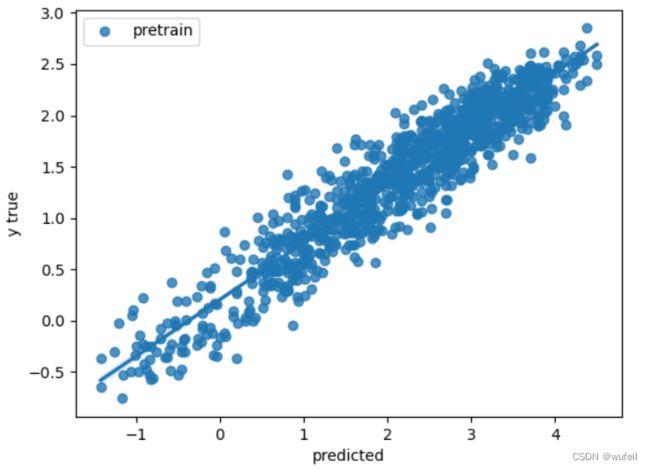
sns.regplot(y_all, y_pred_all, label='pretrain')
plt.ylabel('y true')
plt.xlabel('predicted')
plt.legend()
plt.savefig('Masking_Supervised_Test_curve.png') #保存图片
plt.cla()
plt.clf()
'''
没有预训练的条件下
'''
pre_model = GNN(7,256) #主模型, 参数要和预训练的一致,模型结构先实例化一遍
#线性层
linear_model = Pred_linear(256, 128, 1)
#连成新的模型
model = GNN_graphpred(pre_model=pre_model, pre_model_files='GIN.pth',
graph_pred_linear=linear_model, if_pretrain=False) # if_pretrain控制不使用预训练的权重
model = model.to(device)
optimizer = optim.Adam(model.parameters(), lr=0.001, weight_decay=1e-4)
criterion = torch.nn.MSELoss()
un_log_loss = []
un_log_r2 = []
un_log_corr = []
un_log_loss_test = []
un_log_r2_test = []
un_log_corr_test = []
for epoch in range(1, epoches):
print("====epoch " + str(epoch))
loss, r2, corr, loss_test, r2_test, corr_test = train(model, device, loader_train, loader_test, optimizer, criterion)
un_log_loss.append(loss)
un_log_r2.append(r2)
un_log_corr.append(corr)
un_log_loss_test.append(loss_test)
un_log_r2_test.append(r2_test)
un_log_corr_test.append(corr_test)
print('loss:{:.4f}, r2:{:.4f}, corr:{:.4f}, loss_test:{:.4f}, r2_test:{:.4f}, corr_test:{:.4f}'.format(loss, r2, corr, loss_test, r2_test, corr_test))
#对测试集的预测
y_all = []
y_pred_all = []
for step, batch in enumerate(loader_test):
batch = batch.to(device)
pred = model(batch)
y = batch.y.view(pred.shape).to(torch.float64)
pred = list(pred.detach().cpu().reshape(-1).numpy())
y = list(y.detach().cpu().reshape(-1).numpy())
y_all = y_all + y
y_pred_all = y_pred_all + pred
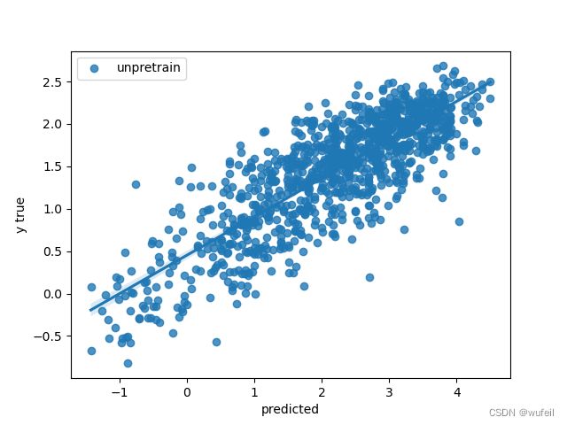
sns.regplot(y_all, y_pred_all, label='unpretrain')
plt.ylabel('y true')
plt.xlabel('predicted')
plt.legend()
plt.savefig('Derectly_Supervised_Test_curve.png') #保存图片
plt.cla()
plt.clf()
'''
保存图片,比较有预训练和没有预训练的差距
'''
plt.figure(figsize=(15,6))
plt.subplot(1,3,1)
plt.plot(log_loss, label='loss')
plt.plot(log_loss_test, label='loss_test')
plt.plot(un_log_loss, label='unpretrain_loss')
plt.plot(un_log_loss_test, label='unpretrain_loss_test')
plt.xlabel('Epoch')
plt.ylabel('MSE Loss')
plt.legend()
plt.subplot(1,3,2)
plt.plot(log_corr, label='corr')
plt.plot(log_corr_test, label='corr_test')
plt.plot(un_log_corr, label='unpretrain_corr')
plt.plot(un_log_corr_test, label='unpretrain_corr_test')
plt.xlabel('Epoch')
plt.ylabel('Corr')
plt.legend()
plt.subplot(1,3,3)
plt.plot(log_r2[1:], label='r2')
plt.plot(log_r2_test[1:], label='r2_test')
plt.plot(un_log_r2[1:], label='unpretrain_r2')
plt.plot(un_log_r2_test[1:], label='unpretrain_r2_test')
plt.ylim(0,1)
plt.xlabel('Epoch')
plt.ylabel('R2')
plt.legend()
plt.savefig('Comversion_Train_process.png')结果如下图。下图是在Lipophilicity数据集上的结果。

200次迭代的训练结果差别还是很大的,预训练提供了很好的性能,相关系数(Corr)超过0.9,而没有预训练的相关系数只有0.8。其实,我也做过2000个迭代的结果,最终结果预训练和没有预训练是一样的。不管怎恶魔说,预训练过程对提升模型泛化能力,和减少训练次数,过拟合,是有帮助的。
七、Grapgh transformer用于Attribute prediction预训练
作为模型的改进,我也考虑过使用更为复杂的模型来进行Attribute prediction预训练,与训练过程就不展示了,直接给出,有预训练和没有预训练的差别。同样是在Lipophilicity数据集上。如下:
差距非常明显。对于复杂的Grapgh transformer模型,如果没有预训练,几乎是没有性能,或者性能非常差。这说明,对于复杂的图神经网络,需要预训练的,否则可能效果更差。
八、代码运行环境及其下载
运行目录结构:
.
├── Comversion_Train_process.png
├── Derectly_Supervised_Test_curve.png
├── Masking_Supervised_Test_curve.png
├── Masking_Supervised_log_train_corr.npy
├── Masking_Supervised_log_train_corr_test.npy
├── Masking_Supervised_log_train_loss.npy
├── Masking_Supervised_log_train_loss_test.npy
├── Masking_Supervised_log_train_r2.npy
├── Masking_Supervised_log_train_r2_test.npy
├── Net_GIN.pth
├── Net_GIN_para.pth
├── Pyg_pretrain.yml
├── dataset
├── linear_pred_atoms.pth
├── linear_pred_bonds.pth
├── log_acc_edge.npy
├── log_acc_node.npy
├── log_loss.npy
├── masking_pretrain.py
├── masking_pretrian_supervised.pth
├── masking_pretrian_supervised_para.pth
├── masking_supervised.py
└── pretrain_masking_预训练损失函数.ipynb执行:python masking_pretrain.py即可进行预训练,随后python masking_supervised.py即可进行随后的图层面面监督学习。
项目的conda环境请见Pyg_pretrain.yml文件。
源代码下载:
链接:https://pan.baidu.com/s/1J9ghAuKpJIFxRz3kn4d5LQ
提取码:7xbi