python风控建模实战（分类器模型+回归模型）

在全球数字经济时代，有一种金融优势，那就是基于消费者大数据的纯信用！

我们不妨称之为数据信用，它是一种面向未来的财产权，它是数字货币背后核心的抵押资产，它决定了数字货币时代信用创造的方向、速度和规模。一句话，谁掌握了数据信用，谁就控制了数字货币的发行权！数据信用判断依靠的就是金融风控模型。

数据信用判断依靠的就是金融风控模型。更准确的说谁能掌握风控模型知识，谁就掌握了数字货币的发行权！

欢迎各位同学学习：

欢迎各位同学学习python风控建模实战lendingClub，链接地址为https://edu.csdn.net/course/detail/30742

 

 

 

 

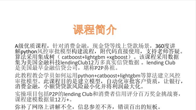
之前博主录制《python信用模型建模（附代码）》课程是针对逻辑回归模型模型；《python风控建模实战lendingClub》此课程是针对集成树模型，包括catboost，lightgbm，xgboost。两个课程算法原理是不同的。

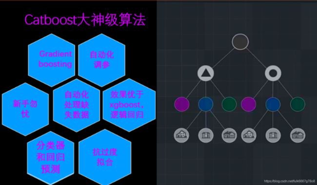
此课程catboost集成树算法有诸多优点，自动化处理缺失数据，自动化调参，无需变量卡方分箱。学员学完后不再为数据预处理，调参，变量分箱而烦恼。此教程建立模型性能卓越，最高性能ks:0.5869,AUC:0.87135，远超互联网上其它建模人员性能。

 

（lendingclub分类器模型数据下载地址）

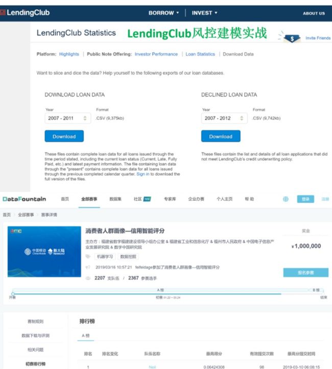
（移动杯消费金融回归模型百万奖金挑战赛数据下载地址）

 

 

 

 

 

 

课程目录

章节1 python编程环境搭建
课时1风控建模语言，python，R，SAS优劣对比
课时2Anaconda快速入门指南
课时3Anaconda下载安装
课时4canopy下载和安装
课时5Anaconda Navigator导航器05:38
课时6python第三方包安装(pip和conda install)
课时7Python非官方扩展包下载地址
课时8Anaconda安装不同版本python
课时9为什么使用jupyter notebook及如何安装
课时10如何用jupyter notebook打开指定文件夹内容？
课时11jupyter基本文本编辑操作
课时12jupyter生成在线PPT汇报文档
课时13jupyter notebook用matplotlib不显示图片解决方案

章节2 python编程基础
课时14Python文件基本操作
课时15python官网
课时16变量_表达式_运算符_值
课时17字符串string
课时18列表list
课时19程序的基本构架（条件，循环）
课时20数据类型_函数_面向对象编程
课时21python2和3区别
课时22编程技巧和学习方法

章节3 python机器学习基础知识
课时23UCI机器学习数据库介绍
课时24机器学习书籍推荐
课时25如何选择算法
课时26sklearn机器学习算法速查表
课时27python数据科学常用的库
课时28python数据科学入门介绍（选修）

章节4 lendingClub业务介绍（P2P鼻祖）
课时29lendingClub业务简介
课时30lendingclub债务危机及深层次时代背景
课时31lendingClub官网数据下载(或本集参考资料下载)

章节5catboost基础介绍
课时32catboost基础知识讲解-比xgboost更优算法登场
课时33catboost官网介绍

章节6 lengding Club实战_catboost分类器模型
课时34数据清洗和首次变量筛选
课时35catboost第三方包下载和安装
课时36import导入建模的包
课时37读取数据和描述性统计
课时38train，test训练和测试数据划分
课时39fit训练模型
课时40模型验证概述
课时41树模型需要相关性检验吗？
课时42交叉验证cross validation
课时43混淆矩阵理论概述，accuracy，sensitivity，precision，F1分数
课时44混淆矩阵python脚本实现
课时45计算模型ks(Kolmogorov-Smirnoff)
课时46catboost1_建模脚本连贯讲解
课时47catboost2_第二次变量筛选
课时48catboost3_分类变量cat_features使用

章节7KS（Kolmogorov–Smirnov）模型区分能力指标
课时49KS简介
课时50step1获取模型分
课时51step2_计算ks_方法1
课时52step3_计算ks_方法2
课时53step4_计算ks_excel推理
课时54step5_绘制KS图
课时55step6_KS评估函数
课时56step7_KS脚本汇总_分治算法
课时57step8_KS缺陷

章节8AUC（Area Under Curve）模型区分能力指标

课时58 ROC基本含义
课时58excel绘制ROC曲
课时59python计算AUC很简单
课时60python轻松绘制ROC曲线
课时61AUC评估函数_AUC多大才算好？
课时62Gini基尼系数基本概念和AUC关系

章节9pickle保存模型
课时63pickle保存和导入模型包_避免重复训练模型时间

章节10PSI模型稳定性评估指标（上）
课时64拿破仑和希特勒征服欧洲为何失败？数学PSI指标揭露历史真相
课时65excel手把手教你推导PSI的计算公式
课时66PSI计算公式奥义
课时67PSI的python脚本讲解

章节11PSI模型稳定性评估指标（下）
课时68step1.筛选lendingClub2018年Q3和Q4数据
课时69step2_计算train，test，oot模型分
课时70step3.计算Q3和Q4模型分PSI

章节12模型维度与边际效应
课时71边际效应基本概念
课时72模型维度与边际效应,变量越多越好吗？
课时73降维实操，结果让人吃惊！
课时74模型变量数量越多，区分能力（ks）越高吗？

章节13catboost分类变量处理
课时75 One-hot encoding热编码
课时76 cat_features分类变量处理（数值型）1
课时77 cat_features分类变量处理（字符串类型）
课时78 不同分类变量处理方法的结果对比

章节14catboost调参
课时79GridSearchCV网格调参简述
课时80iterations树的颗树
课时81eval_metric评估参数（logloss_AUC_Accuracy_F1_Recall）
课时82learning_rate学习率
课时83树深度depth（max_depth）
课时84 l2_leaf_reg正则系数L2调参

章节15多算法比较
课时85xgboost分类器模型
课时86lightgbm分类器建模
课时87逻辑回归分类器和多算法比较结果

章节16消费者信用评分实战_回归模型
课时88机器学习回归竞赛_一百万奖金挑战
课时89线性回归基础知识（最小二乘法OLS）
课时90梯度下降法gradient descent
课时91误差error_偏差bias_方差variance
课时92shrinkage特征缩减技术_正则化
课时93ridge岭回归_lasso回归_elasticNetwork弹性网络
课时94sklearn_ridge岭回归脚本
课时95逻辑回归_regression脚本
课时96支持向量回归SVR脚本
课时97随机森林randomForest回归脚本
课时98xgboost regression回归脚本
课时99catboost regressor回归脚本
课时100lightgbm基础知识讲解
课时101lightgbm regressor回归脚本
课时102sequencial线性模型回归预测脚本

 

 

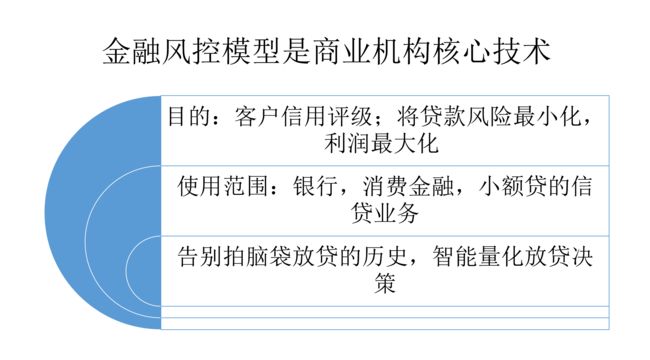
 为什么需要风控模型？

风控模型目的将银行风险最小化并将利润最大化。贷款有风险，如果用户借钱不还或故意骗贷，银行就会有损失。风控模型作用就是识别这些借钱不还用户，然后过滤掉这些坏用户。这样银行放款对象基本是优质客户，可以从中赚取利息，从而达到利润最大化，风险最小化。

为了从银行的角度将损失降到最低，银行需要制定决策规则，确定谁批准贷款，谁不批准。 在决定贷款申请之前，贷款经理会考虑申请人的人口统计和社会经济概况。

 

风控历史

世界上最早的银行出现在意大利。 最早的银行是意大利1407年在威尼斯成立的银行。当然类似于银行的机构可能存更早存在。只要有银行，就会有风险控制和管理，即风控。早期风控包括对借贷人资质审核和账户核实。

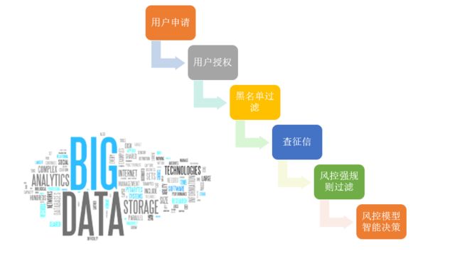
随着金融业发展，贷款流程逐渐完善，包括下图流程

2000-2008后，全球逐步进入大数据时代，随着用户数据整合，诞生央行征信，公安人脸数据，芝麻信用分，同盾分，聚信立蜜罐分，百度黑中介分等参考数据。银行，消费金融公司，小额贷公司可以利用大数据建模，利用机器智能决策代替绝大部分人工审核，缩短信贷流程，减少贷款风险，实现利润最大化。

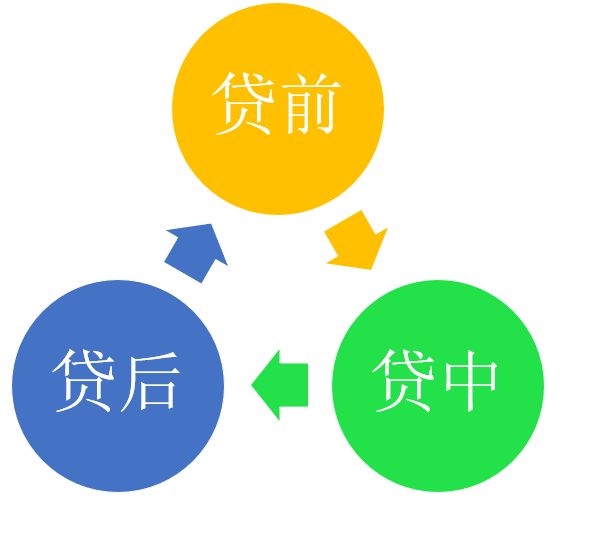
现代大数据时代的风控部门主要分为贷前，贷中和贷后管理三个板块。

信用逾期高发时代

随着我国居民消费心理发生改变和各大商家诱导性消费，不少朋友越来越依赖超前消费了。我国14亿人口，消费群体庞大，各类产品也有着很大的市场，于是现在的消费信贷市场成了很多银行或者其他机构发力的方向。根据央行公布的数据来看，商业银行发行的信用卡数量继续扩张，但在“滥发”信用卡的背后，逾期坏账不断增加也成了银行头疼问题。

信用卡逾期半年以上坏账突破900亿

近日，央行公布了三季度支付体系的运行报告，从央行公布的数据来看，我国商业银行发行的信用卡数量、授信总额以及坏账总额均在保持增长。

数据显示，截至今年三季度末，我国商业银行发行的信用卡（包括借贷合一卡）的数量达到了7.66亿张，环比增加1.29%。总授信额度达到了18.59万亿元，环比增加3.80%。

下卡量在增加，加上授信总额在不断增长，说明银行依旧非常重视信用卡市场，但同时这也给银行带来了不小的麻烦。因为截至今年三季度末，信用卡逾期半年以上的坏账来到了906.63亿元，环比大涨6.13%。

信用卡下卡数量不断增加，说明在初审阶段银行并没有管理的太严格，因此坏账增加是客观会存在的问题。但作为专业的金融机构，银行显然是不会坐视坏账继续涨下去，不然就会影响到银行的正常经营，也会引起监管层的注意。

所以在这种情况下面，商业银行会对已经下卡的客户进行管理，一般是在消费场景以及防范套现上面下功夫。所以为了你不被银行二次风控，从而对你的信用卡封卡降额，一些不合规的刷卡消费最好还是别碰。

银行风控负责人改如何应对持续上升信用卡坏账？作者认为识别坏客户（骗贷和还款能力不足人群）是关键。只有银行精准识别了坏客户，才能显著降低逾期和坏账率。

之前银行是当铺思想，把钱借给有偿还能力的人。这些人群算是优质客群。更糟糕的是但随着量化宽松，财政货币刺激，M2激增，银行，消费金融公司，小额贷公司纷纷把市场目标扩大到次级客户，即偿还能力不足或没有工作的人，这些人还钱风险很高，因此借钱利息也很高。

国内黑产，灰产已经形成庞大产业链条。根据之前同盾公司统计，黑产团队至少上千个，多大为3人左右小团队，100人以上大团队也有几十上百个。这些黑产团队天天测试各大现金贷平台漏洞，可谓专业产品经理。下图是生产虚假号码的手机卡，来自东南亚，国内可用，可最大程度规避国内安全监控，专门为线上平台现金贷诈骗用户准备。如果没有风控能力，就不要玩现金贷这行了。放款犹如肉包打狗有去无回。

举个身边熟悉例子，作者在之前某宝关键词搜索中，可以发现黑产和灰产身影。

关键词：

注册机，短信服务，短信接收，短信验证，app下单，智能终端代接m

黑产市场风起云涌，银行风控负责人改如何应对持续上升信用卡坏账？作者认为识别坏客户（骗贷和还款能力不足人群）是关键。只有银行精准识别了坏客户，才能显著降低逾期和坏账率。如何精准识别坏客户，改课程会手把手教你大家Python信用模型模型，精准捕捉坏客户，此乃风控守护神。

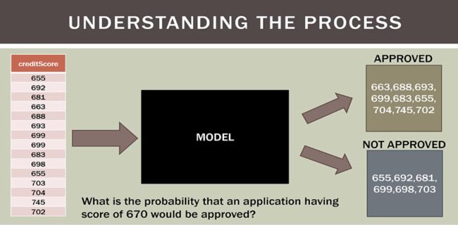
金融风控审批模型可以成为贷款人和借款人计算借款人偿债能力的绝佳工具。对于贷方而言，模型可以帮助他们评估借款人的风险，识别是否是骗贷用户或还款能力不足用户，并帮公司维持健康的投资组合 - 这最终将影响整个经济。

模型就像一个黑箱，当用户申请贷款时，模型会根据用户信息，例如年龄，工作，职位，还款记录，借贷次数等维度自动计算客户坏客户概率。业务线如果用模型计算出某用户坏客户概率较高，例如0.8，就会拒绝改客户贷款申请。

因此风控模型就像信贷守护神，保护公司资产，免受黑产吞噬。模型模型自动化评分，1秒之内决定客户是否通过，贷前人员工作轻松多了！这样，大数据时代下的风控模型就此诞生。

（模型模型自动批量识别坏客户）

第78课，模型训练截图

模型最高性能，ks:0.5869,AUC:0.87135，远超互联网上其它建模人员性能。

 模型降维测试

模型调参测试

接下来，我们展示一下部分python脚本建模和数据分析代码

在课程中，我将研究Lending Club贷款数据，该数据不平衡，大且具有具有不同数据类型的多个功能。 为了进行建模，我将所有违约贷款作为目标变量，并试图预测贷款是否会违约。

导入数据
首先，导入必要的库

import pandas as pd
import numpy as np
import matplotlib.pyplot as plt
import seaborn as sns
sns.set_style('whitegrid')
import warnings
import gc
warnings.simplefilter(action='ignore', category=FutureWarning)
warnings.simplefilter(action='ignore', category=DeprecationWarning)
%matplotlib inline

 导入数据

start_df = pd.read_csv('../input/loan.csv', low_memory=False)

 处理数据的副本，这样我就不必为了节省内存而再次重新读取整个数据集。

df = start_df.copy(deep=True)
df.head()

 

id	member_id	loan_amnt	funded_amnt	funded_amnt_inv	term	int_rate	installment	grade	sub_grade	...	total_bal_il	il_util	open_rv_12m	open_rv_24m	max_bal_bc	all_util	total_rev_hi_lim	inq_fi	total_cu_tl	inq_last_12m
0	1077501	1296599	5000.0	5000.0	4975.0	36 months	10.65	162.87	B	B2	...	NaN	NaN	NaN	NaN	NaN	NaN	NaN	NaN	NaN	NaN
1	1077430	1314167	2500.0	2500.0	2500.0	60 months	15.27	59.83	C	C4	...	NaN	NaN	NaN	NaN	NaN	NaN	NaN	NaN	NaN	NaN
2	1077175	1313524	2400.0	2400.0	2400.0	36 months	15.96	84.33	C	C5	...	NaN	NaN	NaN	NaN	NaN	NaN	NaN	NaN	NaN	NaN
3	1076863	1277178	10000.0	10000.0	10000.0	36 months	13.49	339.31	C	C1	...	NaN	NaN	NaN	NaN	NaN	NaN	NaN	NaN	NaN	NaN
4	1075358	1311748	3000.0	3000.0	3000.0	60 months	12.69	67.79	B	B5	...	NaN	NaN	NaN	NaN	NaN	NaN	NaN	NaN	NaN	NaN

检查数据维度

 

 

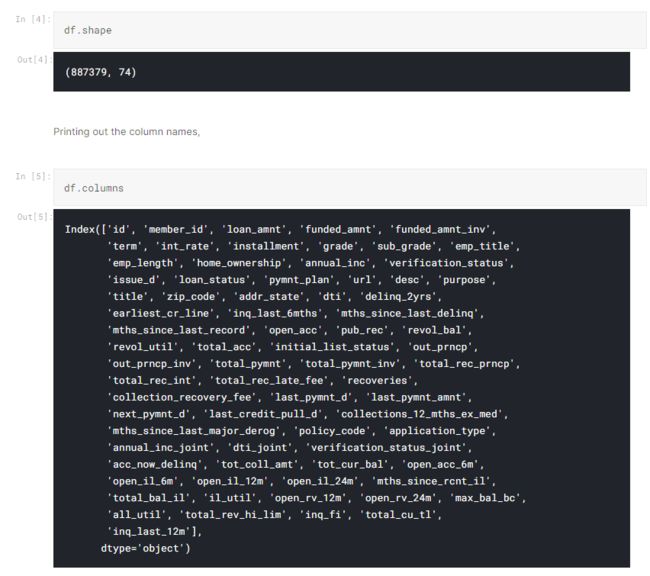
 因此，我们得到很多变量。 知道这些变量的含义可以在以后的建模和数据分析中提供很多帮助。

了解数据
首先，让我们检查数据集中各个列字段的描述。

1 2	df_description = pd.read_excel('../input/LCDataDictionary.xlsx').dropna() df_description.style.set_properties(subset=['Description'], **{'width': '1000px'})

 

LoanStatNew	Description
0	addr_state	The state provided by the borrower in the loan application
1	annual_inc	The self-reported annual income provided by the borrower during registration.
2	annual_inc_joint	The combined self-reported annual income provided by the co-borrowers during registration
3	application_type	Indicates whether the loan is an individual application or a joint application with two co-borrowers
4	collection_recovery_fee	post charge off collection fee
5	collections_12_mths_ex_med	Number of collections in 12 months excluding medical collections
6	delinq_2yrs	The number of 30+ days past-due incidences of delinquency in the borrower's credit file for the past 2 years
7	desc	Loan description provided by the borrower
8	dti	A ratio calculated using the borrower’s total monthly debt payments on the total debt obligations, excluding mortgage and the requested LC loan, divided by the borrower’s self-reported monthly income.
9	dti_joint	A ratio calculated using the co-borrowers' total monthly payments on the total debt obligations, excluding mortgages and the requested LC loan, divided by the co-borrowers' combined self-reported monthly income
10	earliest_cr_line	The month the borrower's earliest reported credit line was opened
11	emp_length	Employment length in years. Possible values are between 0 and 10 where 0 means less than one year and 10 means ten or more years.
12	emp_title	The job title supplied by the Borrower when applying for the loan.*
13	fico_range_high	The upper boundary range the borrower’s FICO at loan origination belongs to.
14	fico_range_low	The lower boundary range the borrower’s FICO at loan origination belongs to.
15	funded_amnt	The total amount committed to that loan at that point in time.
16	funded_amnt_inv	The total amount committed by investors for that loan at that point in time.
17	grade	LC assigned loan grade
18	home_ownership	The home ownership status provided by the borrower during registration. Our values are: RENT, OWN, MORTGAGE, OTHER.
19	id	A unique LC assigned ID for the loan listing.
20	initial_list_status	The initial listing status of the loan. Possible values are – W, F
21	inq_last_6mths	The number of inquiries in past 6 months (excluding auto and mortgage inquiries)
22	installment	The monthly payment owed by the borrower if the loan originates.
23	int_rate	Interest Rate on the loan
24	is_inc_v	Indicates if income was verified by LC, not verified, or if the income source was verified
25	issue_d	The month which the loan was funded
26	last_credit_pull_d	The most recent month LC pulled credit for this loan
27	last_fico_range_high	The upper boundary range the borrower’s last FICO pulled belongs to.
28	last_fico_range_low	The lower boundary range the borrower’s last FICO pulled belongs to.
29	last_pymnt_amnt	Last total payment amount received
30	last_pymnt_d	Last month payment was received
31	loan_amnt	The listed amount of the loan applied for by the borrower. If at some point in time, the credit department reduces the loan amount, then it will be reflected in this value.
32	loan_status	Current status of the loan
33	member_id	A unique LC assigned Id for the borrower member.
34	mths_since_last_delinq	The number of months since the borrower's last delinquency.
35	mths_since_last_major_derog	Months since most recent 90-day or worse rating
36	mths_since_last_record	The number of months since the last public record.
37	next_pymnt_d	Next scheduled payment date
38	open_acc	The number of open credit lines in the borrower's credit file.
39	out_prncp	Remaining outstanding principal for total amount funded
40	out_prncp_inv	Remaining outstanding principal for portion of total amount funded by investors
41	policy_code	publicly available policy_code=1 new products not publicly available policy_code=2
42	pub_rec	Number of derogatory public records
43	purpose	A category provided by the borrower for the loan request.
44	pymnt_plan	Indicates if a payment plan has been put in place for the loan
45	recoveries	post charge off gross recovery
46	revol_bal	Total credit revolving balance
47	revol_util	Revolving line utilization rate, or the amount of credit the borrower is using relative to all available revolving credit.
48	sub_grade	LC assigned loan subgrade
49	term	The number of payments on the loan. Values are in months and can be either 36 or 60.
50	title	The loan title provided by the borrower
51	total_acc	The total number of credit lines currently in the borrower's credit file
52	total_pymnt	Payments received to date for total amount funded
53	total_pymnt_inv	Payments received to date for portion of total amount funded by investors
54	total_rec_int	Interest received to date
55	total_rec_late_fee	Late fees received to date
56	total_rec_prncp	Principal received to date
57	url	URL for the LC page with listing data.
58	verified_status_joint	Indicates if the co-borrowers' joint income was verified by LC, not verified, or if the income source was verified
59	zip_code	The first 3 numbers of the zip code provided by the borrower in the loan application.
60	open_acc_6m	Number of open trades in last 6 months
61	open_il_6m	Number of currently active installment trades
62	open_il_12m	Number of installment accounts opened in past 12 months
63	open_il_24m	Number of installment accounts opened in past 24 months
64	mths_since_rcnt_il	Months since most recent installment accounts opened
65	total_bal_il	Total current balance of all installment accounts
66	il_util	Ratio of total current balance to high credit/credit limit on all install acct
67	open_rv_12m	Number of revolving trades opened in past 12 months
68	open_rv_24m	Number of revolving trades opened in past 24 months
69	max_bal_bc	Maximum current balance owed on all revolving accounts
70	all_util	Balance to credit limit on all trades
71	total_rev_hi_lim	Total revolving high credit/credit limit
72	inq_fi	Number of personal finance inquiries
73	total_cu_tl	Number of finance trades
74	inq_last_12m	Number of credit inquiries in past 12 months
75	acc_now_delinq	The number of accounts on which the borrower is now delinquent.
76	tot_coll_amt	Total collection amounts ever owed
77	tot_cur_bal	Total current balance of all accounts

通过查看列说明，我们可以做的一件好事是找到具有重要性的列，同时找到因缺少信息而多余的列。

让我们还查看缺失值的数量和百分比，

1 2 3 4 5 6 7 8 9 10 11 12 13

def null_values(df):         mis_val = df.isnull().sum()         mis_val_percent = 100 * df.isnull().sum() / len(df)         mis_val_table = pd.concat([mis_val, mis_val_percent], axis=1)         mis_val_table_ren_columns = mis_val_table.rename(         columns = {0 : 'Missing Values', 1 : '% of Total Values'})         mis_val_table_ren_columns = mis_val_table_ren_columns[             mis_val_table_ren_columns.iloc[:,1] != 0].sort_values(         '% of Total Values', ascending=False).round(1)         print ("Dataframe has " + str(df.shape[1]) + " columns.\n"                  "There are " + str(mis_val_table_ren_columns.shape[0]) +               " columns that have missing values.")         return mis_val_table_ren_columns

 

1 2 3

# Missing values statistics miss_values = null_values(df) miss_values.head(20)

 

许多列中丢失数据的百分比远远超出了我们的工作范围。 因此，稍后我们必须删除数据量少于总数据量一定百分比的列。

我们还要检查的另一件事是，与其他贷款相比，有多少贷款处于违约贷款状态。 在此类数据集中进行预测的常见现象是，新贷款是否会违约。 我将使用违约状态的贷款作为目标变量。

1 2 3 4

target_list = [1 if i=='Default' else 0 for i in df['loan_status']]   df['TARGET'] = target_list df['TARGET'].value_counts()

 

 很明显，这是不平衡数据问题的一种情况，其中阶级的价值远远小于另一个。 有用于解决此类问题的基于成本函数的方法和基于抽样的方法，我们稍后将使用它们，以便我们的模型在尝试预测贷款是否会违约时不会表现出高偏差。

 

1	df.drop('loan_status',axis=1,inplace=True)

 然后，查看我们正在使用的数据类型的分布

 因此，我们有很多具有对象数据类型的列，这将在建模时造成问题。
让我们看看具有“对象”数据类型的列包含多少分类数据：

1	df.select_dtypes('object').apply(pd.Series.nunique, axis = 0)

 

 我们希望对仅包含2个分类数据的列进行标签编码，并对超过2个分类数据的一键编码列进行标签编码。 另外，应删除诸如emp_title，url，desc等之类的列，因为它们所包含的任何类别都没有大量唯一数据。 同样，可以对一键编码的列执行主成分分析，以降低特征尺寸。

异常值检测
让我们检查数据中是否存在异常。 通常在处理时间（例如工作年限）的列中发现可能的数据异常。 让我们快速通过它们。

 

1	df['emp_length'].head(3)

 

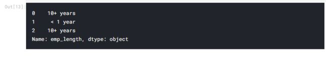
 我将用0填充空值，前提是借款人没有工作很多年才能记录其数据。 另外，我将使用正则表达式从所有数据中提取年数。

1 2 3 4 5 6 7 8

df['emp_length'].fillna(value=0,inplace=True)   df['emp_length'].replace(to_replace='[^0-9]+', value='', inplace=True, regex=True)   df['emp_length'].value_counts().sort_values().plot(kind='barh',figsize=(18,8)) plt.title('Number of loans distributed by Employment Years',fontsize=20) plt.xlabel('Number of loans',fontsize=15) plt.ylabel('Years worked',fontsize=15);

 

 

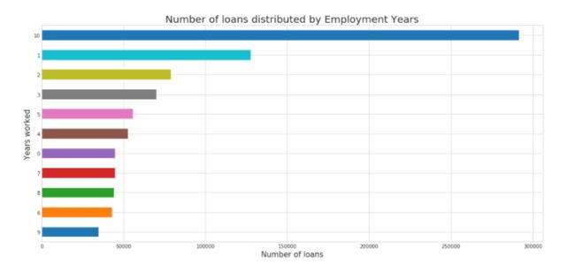
 该变量看起来不错。 此外，可以看出，工作了10年或以上的人更有可能借贷。

1 2 3 4 5

fig = plt.figure(figsize=(12,6)) sns.violinplot(x="TARGET",y="loan_amnt",data=df, hue="pymnt_plan", split=True) plt.title("Payment plan - Loan Amount", fontsize=20) plt.xlabel("TARGET", fontsize=15) plt.ylabel("Loan Amount", fontsize=15);

 

 很正常，违约贷款没有偿还付款计划

探索性数据分析
让我删除所有丢失数据超过70％的列，因为它们对建模和探索无济于事。

 建模
现在，对于建模，我将使用两种集成方法并进行比较。

i）Bootstrap Aggregrating or Bagging

ii）Boosting


1）Bagging - Random Forest
集成决策树算法

通过套袋方法进行培训（重复抽样替换）

装袋：样品中的样品
RF：来自预测变量的样本。 m = sqrt（p）用于分类，m = p / 3用于回归问题。
利用不相关的树

 

1 2 3

from sklearn.ensemble import RandomForestClassifier from sklearn.model_selection import cross_val_score, cross_val_predict from sklearn.metrics import accuracy_score, classification_report, confusion_matrix

 

 创建分类器，

1 2 3 4 5 6 7 8 9 10 11 12 13 14 15 16

#python风控建模实战lendingClub：https://ke.qq.com/course/3063950?tuin=dcbf0baedef print_score(clf, X_train, y_train, X_test, y_test, train=True):     if train:         print("Train Result:\n")         print("accuracy score: {0:.4f}\n".format(accuracy_score(y_train, clf.predict(X_train))))         print("Classification Report: \n {}\n".format(classification_report(y_train, clf.predict(X_train))))         print("Confusion Matrix: \n {}\n".format(confusion_matrix(y_train, clf.predict(X_train))))           res = cross_val_score(clf, X_train, y_train, cv=10, scoring='accuracy')         print("Average Accuracy: \t {0:.4f}".format(np.mean(res)))         print("Accuracy SD: \t\t {0:.4f}".format(np.std(res)))               elif train==False:         print("Test Result:\n")                print("accuracy score: {0:.4f}\n".format(accuracy_score(y_test, clf.predict(X_test))))         print("Classification Report: \n {}\n".format(classification_report(y_test, clf.predict(X_test))))         print("Confusion Matrix: \n {}\n".format(confusion_matrix(y_test, clf.predict(X_test))))

 划分训练数据和测试数据

1	from sklearn.model_selection import train_test_split

 

1	X_train, X_test, y_train, y_test = train_test_split(df.drop('TARGET',axis=1),df['TARGET'],test_size=0.15,random_state=101)

 释放内存

1 2	del start_df gc.collect()

 通过去除均值并缩放到单位方差来标准化特征

1	from sklearn.preprocessing import StandardScaler

sc = StandardScaler()
X_train = sc.fit_transform(X_train)
X_test=sc.transform(X_test)

对训练集进行过采样

1	from imblearn.over_sampling import SMOTE

 现在，我将尝试不同的模型以获得最佳的预测分数。

使用Logistic回归创建准确性和召回率的基准，

 

 准确率和召回得分对基线来说是令人满意的。 但是，精度似乎很差。

对于我们来说，过度拟合将是一个巨大的问题。 因此，我使用的是随机森林，因为它可以通过随机选择要素来减少过拟合。

 

 我们的验证集精度很高，但是召回率却很低。 使用此模型不是一个好主意，因为我们的大多数违约贷款将被错误分类。

2）boosting：
训练弱分类器
通过加权将它们添加到最终的强分类器中。 按精度加权（通常）
添加后，数据将重新加权
错误分类的样本会增加体重
Algo被迫从错误分类的样本中学习更多
为了提高效率，我将使用LightGBM分类器（评估指标为AUC）以及Kfold交叉验证。

1 2 3

from sklearn.metrics import roc_auc_score, roc_curve from sklearn.model_selection import KFold, StratifiedKFold from lightgbm import LGBMClassifier

 结合使用LightGBM和Kfold交叉验证的功能

1 2 3 4 5 6 7 8 9 10 11 12 13 14 15 16 17 18 19 20 21 22 23 24 25 26 27 28 29 30 31 32 33 34 35 36 37 38 39 40 41 42 43 44 45 46 47 48 49 50 51 52 53

#python风控建模实战lendingClub：https://ke.qq.com/course/3063950?tuin=dcbf0baedef kfold_lightgbm(train_df, num_folds, stratified = False):     print("Starting LightGBM. Train shape: {}".format(train_df.shape))           # Cross validation model     if stratified:         folds = StratifiedKFold(n_splits= num_folds, shuffle=True, random_state=47)     else:         folds = KFold(n_splits= num_folds, shuffle=True, random_state=47)       oof_preds = np.zeros(train_df.shape[0])       feature_importance_df = pd.DataFrame()     feats = [f for f in train_df.columns if f not in ['TARGET']]           # Splitting the training set into folds for Cross Validation     for n_fold, (train_idx, valid_idx) in enumerate(folds.split(train_df[feats], train_df['TARGET'])):         train_x, train_y = train_df[feats].iloc[train_idx], train_df['TARGET'].iloc[train_idx]         valid_x, valid_y = train_df[feats].iloc[valid_idx], train_df['TARGET'].iloc[valid_idx]           # LightGBM parameters found by Bayesian optimization         clf = LGBMClassifier(             nthread=4,             n_estimators=10000,             learning_rate=0.02,             num_leaves=32,             colsample_bytree=0.9497036,             subsample=0.8715623,             max_depth=8,             reg_alpha=0.04,             reg_lambda=0.073,             min_split_gain=0.0222415,             min_child_weight=40,             silent=-1,             verbose=-1,             )           # Fitting the model and evaluating by AUC         clf.fit(train_x, train_y, eval_set=[(train_x, train_y), (valid_x, valid_y)],             eval_metric= 'auc', verbose= 1000, early_stopping_rounds= 200)         print_score(clf, train_x, train_y, valid_x, valid_y, train=False)         # Dataframe holding the different features and their importance         fold_importance_df = pd.DataFrame()         fold_importance_df["feature"] = feats         fold_importance_df["importance"] = clf.feature_importances_         fold_importance_df["fold"] = n_fold + 1         feature_importance_df = pd.concat([feature_importance_df, fold_importance_df], axis=0)                   # Freeing up memory         del clf, train_x, train_y, valid_x, valid_y         gc.collect()       display_importances(feature_importance_df)     return feature_importance_df

 用于显示变量重要性

1 2 3 4 5 6 7 8

def display_importances(feature_importance_df_):     cols = feature_importance_df_[["feature", "importance"]].groupby("feature").mean().sort_values(by="importance", ascending=False)[:40].index     best_features = feature_importance_df_.loc[feature_importance_df_.feature.isin(cols)]     plt.figure(figsize=(15, 12))     sns.barplot(x="importance", y="feature", data=best_features.sort_values(by="importance", ascending=False))     plt.title('LightGBM Features (avg over folds)')     plt.tight_layout()     plt.savefig('lgbm_importances.png')

feat_importance = kfold_lightgbm(df, num_folds= 3, stratified= False)

 

如我们所见，LightGBM在获得高精度和高召回率方面做得非常出色。 因此，就我们评估的3个模型而言，该模型是最好的。
为了进一步增强模型，可以进行特征工程。 还可以通过将不同的贷款状态放在一起来使用诸如“好贷款”和“坏贷款”之类的更广泛的术语，以获得更均衡的类别计数，而不是违约/非违约。

 此课程采用catboost对称树算法比LightGBM更不容易过度拟合。

欢迎各位学员报名系列课，学习更多金融建模知识

python金融风控模型模型和数据分析微专业课
https://edu.csdn.net/combo/detail/1927