李宏毅机器学习第二十一周周报GAN理论
文章目录
- week21 Theory behind GAN
- 摘要
- Abstract
- 一、李宏毅机器学习——Theory behind GAN
-
- 1. Generation
-
- 2. 最大似然估计
- 3. Generator
- 3. Discriminator
- 二、文献阅读
-
- 1. 题目
- 2. abstract
- 3. 网络架构
-
- 3.1 Sequence Generative Adversarial Nets
- 3.2 SeqGAN via Policy Gradient
- 3.3 The Generative Model for Sequences
- 3.4 The Discriminative Model for Sequences(CNN)
- 4. 文献解读
-
- 4.1 Introduction
- 4.2 创新点
- 4.3 实验过程
-
- 4.3.1 训练设置
- 4.3.2 实验结果
- 4.3.3 相关实验结果
- 4.4 结论
- 三、实验内容
-
- 1. Pytorch实现CycleGAN
-
- 1.1 任务概况
- 1.2实验代码
-
- 1.2.1 models
- 1.2.2 datasets
- 1.2.3 utils
- 1.2.4 train
- 1.2.5 test
- 2. SeqGAN
-
- 2.1 生成器
- 2.2 分辨器
- 2.3 rollout
- 2.4 target_lstm
- 小结
- 参考文献
week21 Theory behind GAN
摘要
本文主要讨论了GAN的理论知识。本文介绍了在GAN模型之前用于处理生成式任务的最大似然估计。在此基础上,本文分别阐述了生成器与分辨器的原理以及训练目标最大化与JS散度的关系。其次本文展示了题为SeqGAN: Sequence Generative Adversarial Nets with Policy Gradient的论文主要内容。这篇论文提出了SeqGAN,该模型补充了该网络在序列化数据处理领域的空白。该文在中国诗、奥巴马演讲、音乐等数据集上进行实验,从数据角度证明了该网络的优越性。最后,本文基于pytorch实现了CycleGAN并用于解决分类facades数据集的图像转换问题。
Abstract
This article mainly discusses the theoretical knowledge of GAN. This article describes the maximum likelihood estimation that was used to process generative tasks before the GAN model. On this basis, this article expounds the principles of generator and discriminator, and the relationship between training target maximization and JS divergence. Secondly, this paper presents the main content of the paper entitled SeqGAN: Sequence Generative Adversarial Nets with Policy Gradient. This paper proposes SeqGAN, a model that complements the network’s gaps in the field of serialized data processing. This paper carries out experiments on datasets such as Chinese poetry, Obama speeches, music, etc., which proves the superiority of the network from the perspective of data. Finally, this article implements CycleGAN based on pytorch and is used to solve the image transformation problem of classified facades datasets.
一、李宏毅机器学习——Theory behind GAN
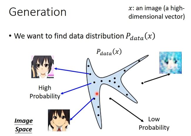
1. Generation
假定如下的分布 P d a t a ( x ) P_{data}(x) Pdata(x)为理想分布,在实线内生成器可以生成理想输出,反之不理想。同时,分布生成的输出落在实线内概率较大,反之较小。而GAN模型的目标是找到这一确定的分布
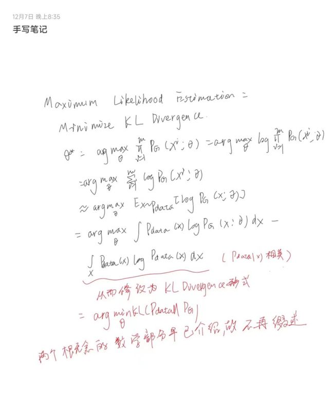
2. 最大似然估计
在GAN模型之前,处理该类任务使用的最大似然估计
对于一个可从中采样的数据分布 P d a t a ( x ) P_{data}(x) Pdata(x),使用由参数 θ \theta θ控制的分布 P G ( x ; θ ) P_G(x;\theta) PG(x;θ)进行拟合。
- 目标是确定一个合适的 θ \theta θ使得拟合分布接近真实分布
- 若拟合分布是一个高斯混合模型,则 θ \theta θ是高斯分布的均值和方差
若 { x 1 , x 2 , … , x m } \{x^1,x^2,\dots,x^m\} {x1,x2,…,xm}是 P d a t a ( x ) P_{data}(x) Pdata(x)中采样获得的样本,则通过这些真实分布的样本可以近似得到多个拟合分布 P G ( x i , θ ) P_G(x^i,\theta) PG(xi,θ)。然后计算各生成样本对应拟合分布的似然性
L = ∏ i = 1 m P G ( x i ; θ ) L=\prod_{i=1}^m P_G(x^i;\theta) L=i=1∏mPG(xi;θ)
确定 θ ∗ \theta^* θ∗使得 a r g max θ ( L ) arg\text{max}_{\theta}(L) argmaxθ(L)
相应的由该式可以推导使得似然估计最大化即使得KL散度最小化(KL散度越小,两个分布相似性越大)
3. Generator
但是当函数不是以高斯函数的形式给出,则无法计算其最大似然估计
由于生成图像所需的真实分布是高维空间的低维映射,所以当使用最大似然估计进行拟合时效果不好。
若生成器G是一个神经网络,该网络定义了概率分布(拟合分布) P G P_G PG
假定由一个正态分布给出z作为生成器G的输入,G根据拟合分布输出 x = G ( z ) x=G(z) x=G(z),目标同样是使得拟合分布与真实分布越近越好。从而有
G ∗ = a r g min g D i v ( P G , P d a t a ) G^*=arg\min_gDiv(P_G,P_{data}) G∗=arggminDiv(PG,Pdata)
即使得两个分布之间的散度最小化。但由于不知道两个分布的形式而仅可从中采样,因此该散度无法计算。
3. Discriminator
将两个分布的采样输入分辨器D,该分辨器产生sigmoid输出,即越接近真实输出分数越大,反之越小。其目标函数为
V ( G , D ) = E x ∼ P d a t a [ l o g D ( x ) ] + E x ∼ P G [ l o g ( 1 − D ( x ) ) ] V(G,D)=E_{x\sim P_{data}}[logD(x)]+E_{x\sim P_G}[log(1-D(x))] V(G,D)=Ex∼Pdata[logD(x)]+Ex∼PG[log(1−D(x))]
在训练过程中G固定,优化D
训练的目标是 D ∗ = a r g max D V ( D , G ) D^*=arg\max_DV(D,G) D∗=argmaxDV(D,G)
在该任务情况下,其与二分类器类似,且目标值的最大化与JS散度相关
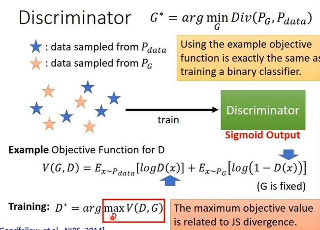
当散度较小时,D难以分辨出数据属于哪个分布,相反当散度较大时,D可以很容易的进行分辨。
以下证明该训练目标的最大化与JS散度相关
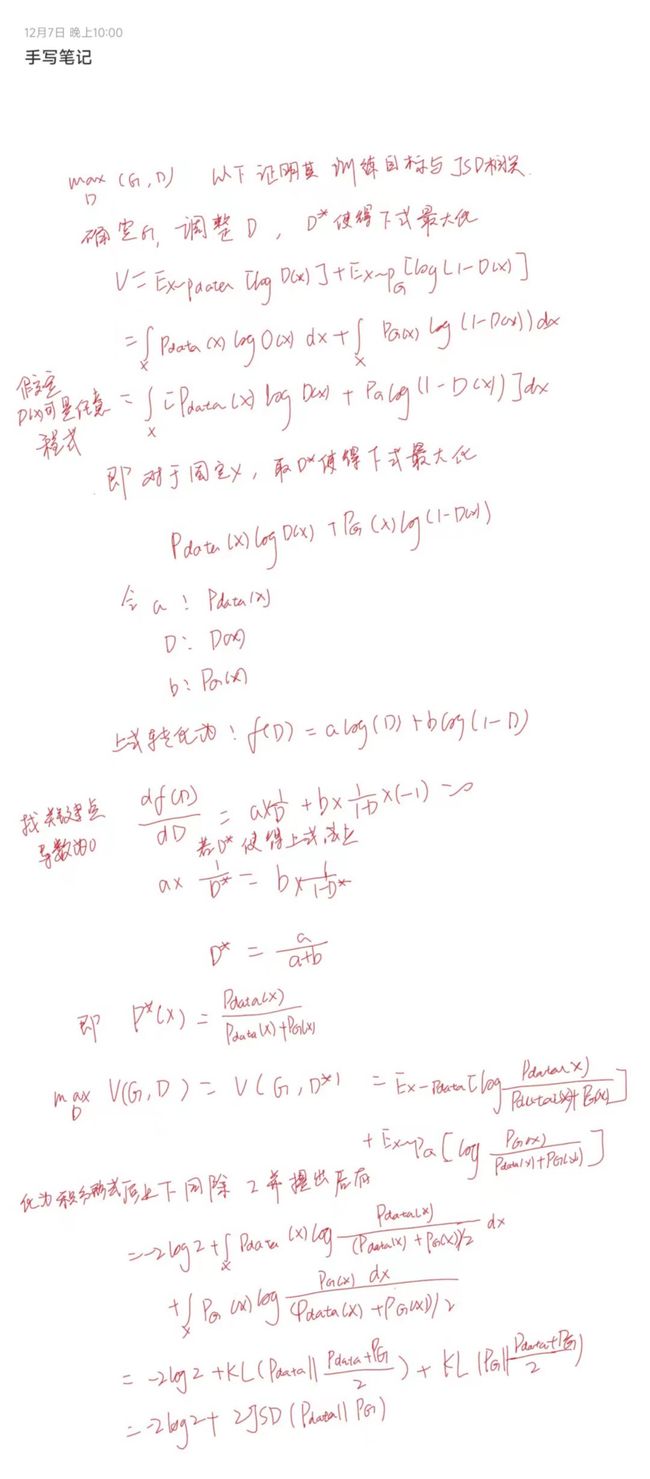
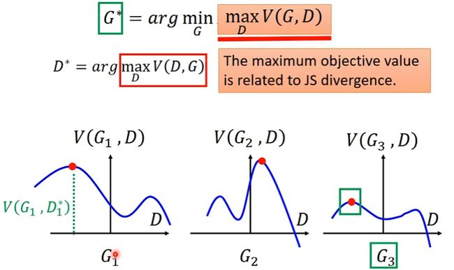
相应的,当训练生成器时,有 G ∗ = a r g min G max D V ( G , D ) G^*=arg\min_G\max_DV(G,D) G∗=argminGmaxDV(G,D)
如下图,假设仅有三种生成器,各生成器与D的图像如下
V(G,D)是拟合分布与真实分布的散度,在下图中为蓝色曲线。而红色点为相对于相应生成器,对应的D取最高值,即此时D最能识别出由该生成器生成的数据与真实数据的区别。
而根据上述目标,显然期望该值越小越好,从而 G 3 G_3 G3是这种情况下最优的生成器,因为其可以使得D在各种情况下取得的V值相较于其他生成器处于较低水平。
二、文献阅读
1. 题目
题目:SeqGAN: Sequence Generative Adversarial Nets with Policy Gradient
作者:Lantao Yu, Weinan Zhang, Jun Wang, Yong Yu
链接:https://arxiv.org/abs/1609.05473
期刊:AAAI2017
2. abstract
该文提出了一个序列生成框架,称为SeqGAN。SeqGAN以强化学习中的随机策略为基础思路重新构建了生成器,通过执行梯度策略绕过生成器微分问题。激励函数源自GAN判别器对完整序列的判断,并使用蒙特卡洛搜索回传中间状态——动作步骤。
This paper proposes a sequence generation framework called SeqGAN. This framework reconstructes the generator based on the stochastic strategy in reinforcement learning, and by passed the generator differentiation problem by executing the gradient strategy. The judgment of the GAN discriminator on the complete sequence controls the reward function. And this framework uses Monte Carlo search to return the intermediate state-action step.
3. 网络架构
3.1 Sequence Generative Adversarial Nets
文本序列生成模型可以表示为,
- 给定真实世界的训练数据集,训练一个生成器 G θ G_\theta Gθ,通过$ G_\theta 来产生序列 来产生序列 来产生序列Y_{1:T}=(y_1,\dots,y_t,\dots,y_T)\in\mathbb Y ,这里 ,这里 ,这里\mathbb Y 表示备选单词的词典。在时间步 t ,状态 s 是当前已经生成的单词序列 表示备选单词的词典。在时间步t ,状态s是当前已经生成的单词序列 表示备选单词的词典。在时间步t,状态s是当前已经生成的单词序列(y_1,\dots,y_t,\dots,y_T) ,动作 a 是下一个将要选择的单词 ,动作a是下一个将要选择的单词 ,动作a是下一个将要选择的单词y_t$ 。故策略模型 G θ ( y t ∣ Y 1 : t − 1 ) G_\theta(y_t|Y_{1:t-1}) Gθ(yt∣Y1:t−1)是随机的,但在选择一个动作之后,状态转移是确定的
- 例如当当前状态是 s = Y 1 : t − 1 s=Y_{1:t-1} s=Y1:t−1, δ s , s ′ a = 1 \delta_{s,s'}^a=1 δs,s′a=1的下一步是 s ′ = Y 1 : t s'=Y_{1:t} s′=Y1:t,而动作 a = y t a=y_t a=yt的下一状态是 s ′ ′ , δ s , s ′ ′ a = 0 s'',\delta_{s,s''}^a=0 s′′,δs,s′′a=0
- 如下图所示,训练一个 ϕ \phi ϕ参数化判别模型 D ϕ D_\phi Dϕ,为改进 G ϕ G_\phi Gϕ提供指导。 D ϕ ( Y 1 : T ) D_\phi(Y_{1:T}) Dϕ(Y1:T)是表示序列 Y 1 : T Y_{1:T} Y1:T是否来自真实序列数据的概率。如下图所示,通过从实际序列数据中提供正面实例和从生成模型 G θ G_\theta Gθ生成的合成序列中提供负面示例来训练判别模型 D θ D_\theta Dθ。同时,根据判别模型 D ϕ D_\phi Dϕ得到的期望最终reward,采用策略梯度和MC搜索对生成模型进行更新。通过欺骗判别模型 D ϕ D_\phi Dϕ的可能性来估计reward
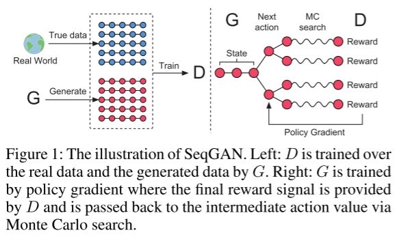
上图左侧:D是G对实际数据和生成的数据进行训练。
上图右侧:G通过策略梯度进行训练,最终的奖励信号由D提供,并通过蒙特卡罗搜索传回中间动作值。
3.2 SeqGAN via Policy Gradient
当没有中间状态时,生成器模型 G θ ( y t ∣ Y 1 : t − 1 ) G_\theta(y_t|Y_{1:t-1}) Gθ(yt∣Y1:t−1)的目的是从起始状态 s 0 s_0 s0生成一个序列,以使其预测的最终预期结果最大化:
J ( θ ) = E [ R T ∣ s 0 , θ ] = ∑ y 1 ∈ Y G θ ( y 1 ∣ s 0 ) ⋅ Q D ϕ G θ ( s 0 , y 1 ) (1) J(\theta)=\mathbb E[R_T|s_0,\theta]=\sum_{y_1\in \mathcal Y}G_\theta(y_1|s_0)\cdot Q_{D_\phi}^{G_\theta}(s_0,y_1) \tag{1} J(θ)=E[RT∣s0,θ]=y1∈Y∑Gθ(y1∣s0)⋅QDϕGθ(s0,y1)(1)
其中 R T R_T RT是对完整序列的激励。
奖励来自于鉴别器 D ϕ D_\phi Dϕ, Q G θ D θ ( s , a ) Q_{G_\theta}^{D_\theta}(s,a) QGθDθ(s,a)是一个序列的动作——值函数,即从状态s开始,采取动作a,然后遵循策略 G θ G_\theta Gθ的期望累计报酬。序列目标函数的合理性在于,从给定初始状态开始,生成器的目标是生成一个使得鉴别器认为是真的序列。
Q G θ D θ ( a = y T , s = Y 1 : T − 1 ) = D ϕ ( Y 1 : T ) (2) Q_{G_\theta}^{D_\theta}(a=y_T,s=Y_{1:T-1})=D_{\phi}(Y_{1:T}) \tag{2} QGθDθ(a=yT,s=Y1:T−1)=Dϕ(Y1:T)(2)
对于一个完整的序列相应的提供完整的激励。由于需要兼顾长期序列的稳定性,在每一步考虑之前token的适合性的同时,考虑将来的状态。进一步的,为了评估中间状态的操作值,应用MTCsearch和推理策略 G β G_\beta Gβ来抽样未知的最后 T t T_t Tt各token。将N次的蒙特卡罗搜索表示为
{ Y 1 : T 1 , … , Y 1 : T N } = MC G β ( Y 1 : t ; N ) (3) \{Y_{1:T}^1,\dots,Y_{1:T}^N\}=\text{MC}^{G_\beta}(Y_{1:t};N) \tag{3} {Y1:T1,…,Y1:TN}=MCGβ(Y1:t;N)(3)
综上,有下述公式
Q G θ D θ ( a = y T , s = Y 1 : T − 1 ) = { 1 N ∑ n = 1 N D ϕ ( Y 1 : T N ) , Y 1 : T ∈ MC G β ( Y 1 : t ; N ) for t < Y , D ϕ ( Y 1 : t ) for t = T (4) Q_{G_\theta}^{D_\theta}(a=y_T,s=Y_{1:T-1})=\\ \begin{cases} \frac1N\sum_{n=1}^ND_\phi(Y_{1:T}^N),Y_{1:T}\in \text{MC}^{G_\beta}(Y_{1:t};N)\quad \text{for}\ t
其中当无中间状态时,该函数从状态 s ′ = Y 1 : t s'=Y_{1:t} s′=Y1:t开始进行推理。
注:若当前序列已经完整,则生成器使用循环神经网络,此时直接将该序列作为分辨器的输入。若当前序列未完整,则使用蒙特卡洛搜索。即使用已经生成的序列,从当前位置的下一个开始采样,得到完整序列,即roll-out policy。该策略通过神经网络实现,该圣经网络即生成器。之后,在将该生成器的输出作为分辨器的输入。
使用判别器 D ϕ D_\phi Dϕ作为激励函数的优点是其可以动态更新,以迭代的改进生成模型。一旦有了一组更真实的生成序列,将重新训练鉴别器模型
min ϕ E Y ∼ p d a t a [ log D ϕ ( Y ) ] − E Y ∼ G θ [ log ( 1 − D ϕ ( Y ) ) ] (5) \min_\phi\mathbb E_{Y\sim p_{data}}[\log D_\phi(Y)]-\mathbb E_{Y\sim G_\theta}[\log(1-D_\phi(Y))] \tag{5} ϕminEY∼pdata[logDϕ(Y)]−EY∼Gθ[log(1−Dϕ(Y))](5)
每次更新判断器模型时,准备更新生成器。所提出的基于策略的优化参数优化策略来最直接最大化长期结果。目标函数 J ( θ ) J(\theta) J(θ)的梯度生成器的参数 θ \theta θ可以推导为
∇ θ J ( θ ) = ∑ t = 1 T E Y 1 : t − 1 ∼ G θ [ ∑ y t ∈ Y ∇ θ G θ ( y t ∣ Y 1 : t − 1 ) ⋅ Q D ϕ G θ ( Y 1 : t − 1 , y t ) ] (6) \nabla_\theta J(\theta)=\sum_{t=1}^T\mathbb E_{Y_{1:t-1\sim G_\theta}}[\sum_{y_t\in \mathcal Y}\nabla_\theta G_\theta(y_t|Y_{1:t-1})\cdot Q_{D_\phi}^{G_\theta}(Y_{1:t-1,y_t})] \tag{6} ∇θJ(θ)=t=1∑TEY1:t−1∼Gθ[yt∈Y∑∇θGθ(yt∣Y1:t−1)⋅QDϕGθ(Y1:t−1,yt)](6)
推导过程如下
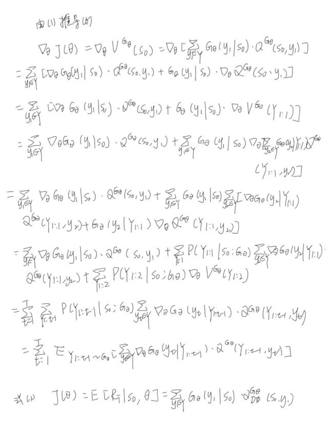
上述形式是基于确定性状态转换和无中间状态产生的。下式为上式的无偏差估计
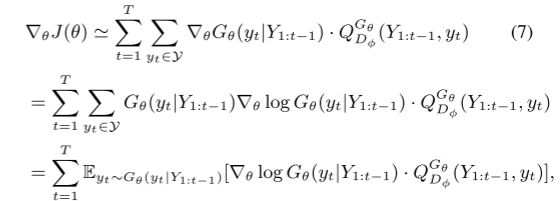
其中 Y 1 : t − 1 Y_{1:t-1} Y1:t−1从 G θ G_\theta Gθ采样的中间状态。期望 E [ ⋅ ] \mathbb E[\cdot] E[⋅]可以通过采样方法来近似,故将生成器的参数更新为
θ ← θ + α h ∇ θ J ( θ ) (8) \theta\leftarrow \theta+\alpha_h\nabla_\theta J(\theta) \tag{8} θ←θ+αh∇θJ(θ)(8)
其中 α h ∈ R + \alpha_h\in \mathbb R^+ αh∈R+表示第h步对应的学习率。此外,其还可以采样Adam或者RMSprop等算法
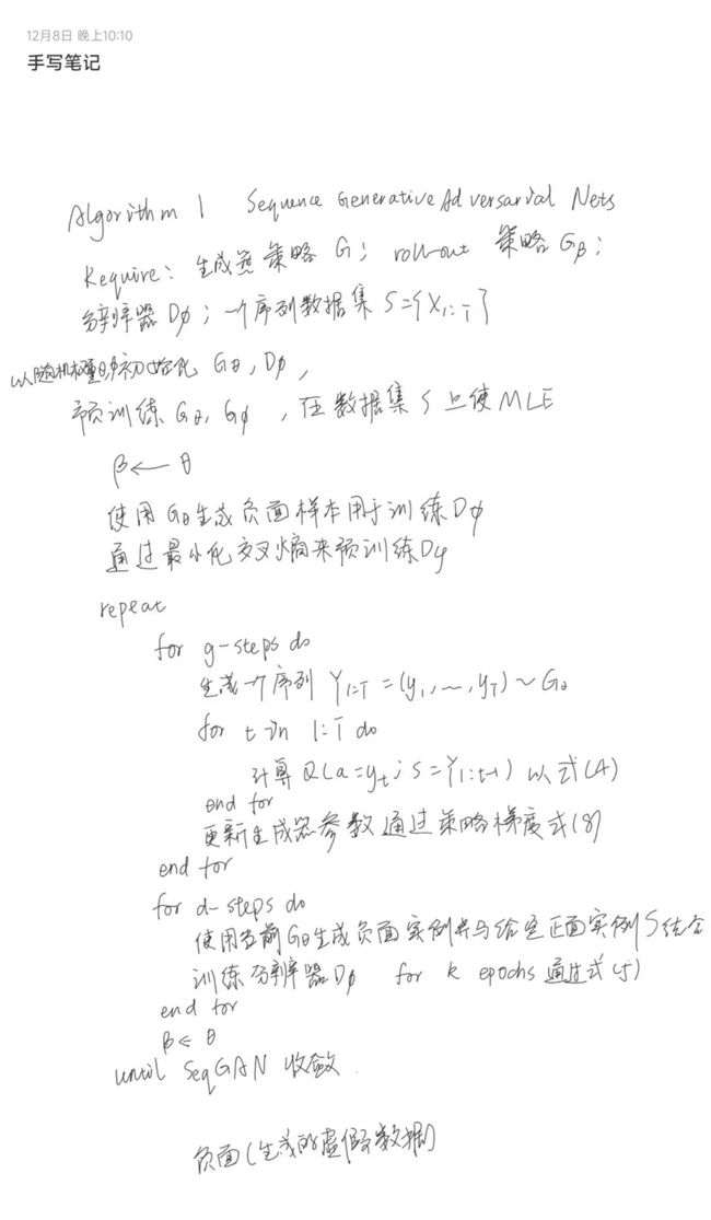
下图中的算法1展示了所提出的SeqGAN的完整细节。在训练开始时,使用最大似然估计来与训练 G θ G_\theta Gθ的训练集S。论文作者发现来自与训练鉴别器的监督信号提供了丰富信息,有助于有效的调整生成器。
3.3 The Generative Model for Sequences
使用递归神经网络作为生成器模型(LSTM)。RNN映射序列输入嵌入表示 x 1 , … , x T x_1,\dots,x_T x1,…,xT。通过递归的使用更新函数g, x 1 , … , x T x_1,\dots,x_T x1,…,xT转换成一系列隐藏状态 h t h_t ht
h t = g ( h t − 1 , x t ) (9) h_t=g(h_{t-1},x_t) \tag{9} ht=g(ht−1,xt)(9)
softmax输出层z将隐藏状态映射至输出token分布(0-1)中:(bias:c,weight:V)
p ( y t ∣ x 1 , … , x t ) = z ( h t ) = softmax ( c + V h t ) (10) p(y_t|x_1,\dots, x_t)=z(h_t)=\text{softmax}(c+Vh_t) \tag{10} p(yt∣x1,…,xt)=z(ht)=softmax(c+Vht)(10)
3.4 The Discriminative Model for Sequences(CNN)
输入序列
E 1 : T = x 1 ⊕ x 2 ⊕ ⋯ ⊕ x T (11) \mathcal E_{1:T}=x_1\oplus x_2\oplus\dots\oplus x_T \tag{11} E1:T=x1⊕x2⊕⋯⊕xT(11)
x是k维的, ⊕ \oplus ⊕表示链接
E 1 : T ∈ R T × k \mathcal E_{1:T}\in \mathbb R_{T\times k} E1:T∈RT×k
一个核 w ∈ R l × k w\in \mathbb R^{l\times k} w∈Rl×k
特征提取:
c i = ρ ( w ⊗ E i : i + l − 1 + b ) (12) c_i=\rho(w\otimes \mathcal E_{i:i+l-1}+b) \tag{12} ci=ρ(w⊗Ei:i+l−1+b)(12)
ρ \rho ρ为非线性函数,b即bias
采用最大池化
c ~ = max c 1 , … , c T − l + 1 \tilde c=\max{c_1,\dots,c_{T-l+1}} c~=maxc1,…,cT−l+1
使用一个具有sigmoid激活的全连接层来输出输入序列是真实的概率。优化目标是最小化地面真实性标签与式(5)中所述预测概率之间的交叉熵
4. 文献解读
4.1 Introduction
生成模仿真实数据的序列合成数据是无监督学习中的一个重要问题。对于GAN而言,首先该模型旨在生成数值、连续数据,但在直接生成离散标记序列方面存在困难。这是由于GAN生成器从随机采样开始,然后进行模型参数控制的确定性变换。其次GAN只能用于在生成整个序列时给出其损失;对于部分生成的序列,平衡整个序列的损失和未来的情况并非易事。
SeqGAN将序列生成问题看成序列决策过程,将目前已经生成的token看为状态(state),将下一个将要生成token看为动作(action),使用判别器来对整个序列做出评估指导生成器学习。为了解决梯度很难传递给生成器的问题,将生成器看为随机策略。在策略梯度中,使用MCT搜索来近似状态-动作对的值。
4.2 创新点
- 解决了使用GAN生成序列的过程中所遇到的两个问题(见introduce),即在策略梯度中采样MCT搜索
- 提出了用于生成序列的新框架seqGAN
4.3 实验过程
4.3.1 训练设置
为了设置合成数据实验,我们首先初始化遵循正态分布 N(0, 1) 的 LSTM 网络参数,作为描述真实数据分布 G o r a c l e ( x t ∣ x 1 , . . . , x t − 1 ) G_{oracle}(x_t|x_1, ..., x_{t−1}) Goracle(xt∣x1,...,xt−1) 的预测器。然后用它生成 10,000 个长度为 20 的序列作为生成模型的训练集 S。
在SeqGAN算法中,判别器的训练集由生成的标签为0的实例和来自S的标签为1的实例组成。对于不同的任务,应该为卷积层设计特定的结构,在合成数据实验中,内核大小从 1 到 T,每个内核大小的数量在 100 到 2003 之间。使用 Dropout和 L2 正则化来避免过度拟合
将四种生成模型与 SeqGAN 进行了比较。
- 随机token生成。
- 经过 MLE 训练的 LSTM G θ G_\theta Gθ。
- 计划抽样(Bengio et al. 2015)[2]。
- BLEU 策略梯度(PG-BLEU)。在计划采样中,训练过程逐渐从完全引导的方案(将真实的先前标记输入 LSTM)转变为较少引导的方案(主要将其生成的标记输入 LSTM)。学习率 ω 用于控制用生成的token替换真实token的概率。为了获得良好且稳定的性能,我们在每个训练周期将 ω 减少 0.002。在 PG-BLEU 算法中,使用 BLEU(一种测量生成序列和参考(训练数据)之间相似性的指标)对蒙特卡罗搜索的最终样本进行评分。
4.3.2 实验结果
下表中以 N L L o r a c l e NLL_{oracle} NLLoracle为指标比较策略生成序列的性能,该文模型有显著改进
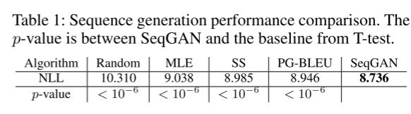
下图为SeqGAN学习曲线,最大似然估计和调度采样方法都收敛到相对较高的 N L L o r a c l e NLL_{oracle} NLLoracle分数,而 SeqGAN 可以显着提高与基线相同结构的生成器的极限。
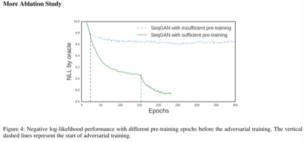
此外,SeqGAN 优于 PG-BLEU,这意味着 GAN 中的判别信号比预定义分数(例如 BLEU)更普遍、更有效,可以指导生成策略捕获序列数据的底层分布。
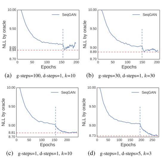
下图显示了调整参数g-steps、d-steps、k对该算法的影响
4.3.3 相关实验结果
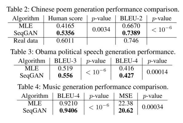
使用 BLEU 分数作为评估指标来衡量生成文本与人工创建文本之间的相似程度
具体来说,对于诗歌评估,将 n-gram 设置为 2 (BLEU-2),因为中国古典诗歌中的大多数单词(依赖)由一个或两个字符组成 (Yi, Li, and Sun 2016),出于类似的原因,使用 BLEU-3 和 BLEU-4 来评估奥巴马语音生成性能。
除了 BLEU 之外,还选择诗歌生成作为人类判断的案例
然后由70人来评判这60首诗中的每一首是人类还是机器创作的。一旦被认为是真实的,则获得+1分,否则为0分。最后,计算每个算法的平均分。
本模型相较于MLE有明显提升
4.4 结论
该文提出了一种序列生成方法 SeqGAN,可以有效地训练生成对抗网络,通过策略梯度生成结构化序列。在合成数据实验中,使用了预测器评估机制来明确说明 SeqGAN 相对于基础模型的优越性。对于诗歌、语音和音乐生成这三个现实场景,SeqGAN 在生成创意序列方面表现出了出色的性能。此外,还进行了一组实验来研究训练 SeqGAN 的鲁棒性和稳定性。
三、实验内容
1. Pytorch实现CycleGAN
1.1 任务概况
任务要求:使用pytorch实现CycleGAN并使用facades数据集训练模型生成图像
本次仅训练了10个epoch,以下第二张图为原图,第三张为实际转换后的结果,而第一张是网络生成的结果


1.2实验代码
1.2.1 models
主要就是设置一个初始化参数的函数,在开始训练时调用。
构建了生成器和判别器网络。
生成器中的残差块除了减弱梯度消失外,还可以理解为这是一种自适应深度,也就是网络可以自己调节层数的深浅,至少可以退化为输入,不会变得更糟糕。可以使网络变得更深,更加的平滑,使深度神经网络的训练成为了可能。
import torch.nn as nn
import torch.nn.functional as F
import torch

## 定义参数初始化函数
def weights_init_normal(m):
    classname = m.__class__.__name__                        ## m作为一个形参,原则上可以传递很多的内容, 为了实现多实参传递,每一个moudle要给出自己的name. 所以这句话就是返回m的名字.
    if classname.find("Conv") != -1:                        ## find():实现查找classname中是否含有Conv字符,没有返回-1;有返回0.
        torch.nn.init.normal_(m.weight.data, 0.0, 0.02)     ## m.weight.data表示需要初始化的权重。nn.init.normal_():表示随机初始化采用正态分布,均值为0,标准差为0.02.
        if hasattr(m, "bias") and m.bias is not None:       ## hasattr():用于判断m是否包含对应的属性bias, 以及bias属性是否不为空.
            torch.nn.init.constant_(m.bias.data, 0.0)       ## nn.init.constant_():表示将偏差定义为常量0.
    elif classname.find("BatchNorm2d") != -1:               ## find():实现查找classname中是否含有BatchNorm2d字符,没有返回-1;有返回0.
        torch.nn.init.normal_(m.weight.data, 1.0, 0.02)     ## m.weight.data表示需要初始化的权重. nn.init.normal_():表示随机初始化采用正态分布,均值为0,标准差为0.02.
        torch.nn.init.constant_(m.bias.data, 0.0)           ## nn.init.constant_():表示将偏差定义为常量0.


##############################
##  残差块儿ResidualBlock
##############################
class ResidualBlock(nn.Module):
    def __init__(self, in_features):
        super(ResidualBlock, self).__init__()

        self.block = nn.Sequential(                     ## block = [pad + conv + norm + relu + pad + conv + norm]
            nn.ReflectionPad2d(1),                      ## ReflectionPad2d():利用输入边界的反射来填充输入张量
            nn.Conv2d(in_features, in_features, 3),     ## 卷积
            nn.InstanceNorm2d(in_features),             ## InstanceNorm2d():在图像像素上对HW做归一化,用在风格化迁移
            nn.ReLU(inplace=True),                      ## 非线性激活
            nn.ReflectionPad2d(1),                      ## ReflectionPad2d():利用输入边界的反射来填充输入张量
            nn.Conv2d(in_features, in_features, 3),     ## 卷积
            nn.InstanceNorm2d(in_features),             ## InstanceNorm2d():在图像像素上对HW做归一化,用在风格化迁移
        )

    def forward(self, x):                               ## 输入为 一张图像
        return x + self.block(x)                        ## 输出为 图像加上网络的残差输出


##############################
##  生成器网络GeneratorResNet
##############################
class GeneratorResNet(nn.Module):
    def __init__(self, input_shape, num_residual_blocks):   ## (input_shape = (3, 256, 256), num_residual_blocks = 9)
        super(GeneratorResNet, self).__init__()

        channels = input_shape[0]                           ## 输入通道数channels = 3

        ## 初始化网络结构
        out_features = 64                                   ## 输出特征数out_features = 64
        model = [                                           ## model = [Pad + Conv + Norm + ReLU]
            nn.ReflectionPad2d(channels),                   ## ReflectionPad2d(3):利用输入边界的反射来填充输入张量
            nn.Conv2d(channels, out_features, 7),           ## Conv2d(3, 64, 7)
            nn.InstanceNorm2d(out_features),                ## InstanceNorm2d(64):在图像像素上对HW做归一化,用在风格化迁移
            nn.ReLU(inplace=True),                          ## 非线性激活
        ]
        in_features = out_features                          ## in_features = 64

        ## 下采样,循环2次
        for _ in range(2):
            out_features *= 2                                                   ## out_features = 128 -> 256
            model += [                                                          ## (Conv + Norm + ReLU) * 2
                nn.Conv2d(in_features, out_features, 3, stride=2, padding=1),
                nn.InstanceNorm2d(out_features),
                nn.ReLU(inplace=True),
            ]
            in_features = out_features                                          ## in_features = 256

        # 残差块儿,循环9次
        for _ in range(num_residual_blocks):
            model += [ResidualBlock(out_features)]                              ## model += [pad + conv + norm + relu + pad + conv + norm]

        # 上采样两次
        for _ in range(2):
            out_features //= 2                                                  ## out_features = 128 -> 64
            model += [                                                          ## model += [Upsample + conv + norm + relu]
                nn.Upsample(scale_factor=2),
                nn.Conv2d(in_features, out_features, 3, stride=1, padding=1),
                nn.InstanceNorm2d(out_features),
                nn.ReLU(inplace=True),
            ]
            in_features = out_features                                          ## out_features = 64

        ## 网络输出层                                                            ## model += [pad + conv + tanh]
        model += [nn.ReflectionPad2d(channels), nn.Conv2d(out_features, channels, 7), nn.Tanh()]    ## 将(3)的数据每一个都映射到[-1, 1]之间

        self.model = nn.Sequential(*model)

    def forward(self, x):           ## 输入(1, 3, 256, 256)
        return self.model(x)        ## 输出(1, 3, 256, 256)


##############################
#        Discriminator
##############################
class Discriminator(nn.Module):
    def __init__(self, input_shape):
        super(Discriminator, self).__init__()

        channels, height, width = input_shape                                       ## input_shape:(3, 256, 256)

        # Calculate output shape of image discriminator (PatchGAN)
        self.output_shape = (1, height // 2 ** 4, width // 2 ** 4)                  ## output_shape = (1, 16, 16)

        def discriminator_block(in_filters, out_filters, normalize=True):           ## 鉴别器块儿
            """Returns downsampling layers of each discriminator block"""
            layers = [nn.Conv2d(in_filters, out_filters, 4, stride=2, padding=1)]   ## layer += [conv + norm + relu]
            if normalize:                                                           ## 每次卷积尺寸会缩小一半,共卷积了4次
                layers.append(nn.InstanceNorm2d(out_filters))
            layers.append(nn.LeakyReLU(0.2, inplace=True))
            return layers

        self.model = nn.Sequential(
            *discriminator_block(channels, 64, normalize=False),        ## layer += [conv(3, 64) + relu]
            *discriminator_block(64, 128),                              ## layer += [conv(64, 128) + norm + relu]
            *discriminator_block(128, 256),                             ## layer += [conv(128, 256) + norm + relu]
            *discriminator_block(256, 512),                             ## layer += [conv(256, 512) + norm + relu]
            nn.ZeroPad2d((1, 0, 1, 0)),                                 ## layer += [pad]
            nn.Conv2d(512, 1, 4, padding=1)                             ## layer += [conv(512, 1)]
        )

    def forward(self, img):             ## 输入(1, 3, 256, 256)
        return self.model(img)          ## 输出(1, 1, 16, 16)


# ## test
# img_shape = (3, 256, 256)
# n_residual_blocks = 9
# G_AB = GeneratorResNet(img_shape, n_residual_blocks)
# D_A = Discriminator(img_shape)
# img = torch.rand((1, 3, 256, 256))
# fake = G_AB(img)
# print(fake.shape)

# fake_D = D_A(img)
# print(fake_D.shape)
1.2.2 datasets
其中的root代表着存放的文件夹,命名格式如:./datasets/facades
调用train_data_loader()函数即可,得到的是字典格式的数据,可以通过data[‘A’],和data[‘B’]操作将不同类型的图片取出来。
import glob
import random
import os
from torch.utils.data import Dataset
from PIL import Image
import torchvision.transforms as transforms

## 如果输入的数据集是灰度图像,将图片转化为rgb图像(本次采用的facades不需要这个)
def to_rgb(image):
    rgb_image = Image.new("RGB", image.size)
    rgb_image.paste(image)
    return rgb_image


## 构建数据集
class ImageDataset(Dataset):
    def __init__(self, root, transforms_=None, unaligned=False, mode="train"):          ## (root = "./datasets/facades", unaligned=True:非对其数据)
        self.transform = transforms.Compose(transforms_)                                ## transform变为tensor数据
        self.unaligned = unaligned

        self.files_A = sorted(glob.glob(os.path.join(root, "%sA" % mode) + "/*.*"))     ## "./datasets/facades/trainA/*.*"
        self.files_B = sorted(glob.glob(os.path.join(root, "%sB" % mode) + "/*.*"))     ## "./datasets/facades/trainB/*.*"

    def __getitem__(self, index):
        image_A = Image.open(self.files_A[index % len(self.files_A)])                   ## 在A中取一张照片

        if self.unaligned:                                                              ## 如果采用非配对数据,在B中随机取一张
            image_B = Image.open(self.files_B[random.randint(0, len(self.files_B) - 1)])
        else:
            image_B = Image.open(self.files_B[index % len(self.files_B)])

        # 如果是灰度图,把灰度图转换为RGB图
        if image_A.mode != "RGB":
            image_A = to_rgb(image_A)
        if image_B.mode != "RGB":
            image_B = to_rgb(image_B)

        # 把RGB图像转换为tensor图, 方便计算,返回字典数据
        item_A = self.transform(image_A)
        item_B = self.transform(image_B)
        return {"A": item_A, "B": item_B}

    ## 获取A,B数据的长度
    def __len__(self):
        return max(len(self.files_A), len(self.files_B))
1.2.3 utils
这个模块设计了一个缓冲区,和学习率更新的函数
在更新discriminators的时候,用的是之前生成的图片,而不是最新的图片,所以设立图片缓冲区,可以存放50张之前生成的图片。
学习率初始为0.0003,总的epoch为50,在0-30的时候,学习率为0.0003,在30-50的时候,学习率逐渐线性减小为0,所以需要进行学习率的更新。
需要的变量有:总的训练epoch,当前的epoch,和开始进行衰减的epoch,即可实现lr的线性变化。
import random
import time
import datetime
import sys
from torch.autograd import Variable
import torch
import numpy as np
from torchvision.utils import save_image

## 先前生成的样本的缓冲区
class ReplayBuffer:
    def __init__(self, max_size=50):
        assert max_size > 0, "Empty buffer or trying to create a black hole. Be careful."
        self.max_size = max_size
        self.data = []

    def push_and_pop(self, data):                       ## 放入一张图像,再从buffer里取一张出来
        to_return = []                                  ## 确保数据的随机性,判断真假图片的鉴别器识别率
        for element in data.data:
            element = torch.unsqueeze(element, 0)
            if len(self.data) < self.max_size:          ## 最多放入50张,没满就一直添加
                self.data.append(element)
                to_return.append(element)
            else:
                if random.uniform(0, 1) > 0.5:          ## 满了就1/2的概率从buffer里取,或者就用当前的输入图片
                    i = random.randint(0, self.max_size - 1)
                    to_return.append(self.data[i].clone())
                    self.data[i] = element
                else:
                    to_return.append(element)
        return Variable(torch.cat(to_return))


## 设置学习率为初始学习率乘以给定lr_lambda函数的值
class LambdaLR:
    def __init__(self, n_epochs, offset, decay_start_epoch):                                                ## (n_epochs = 50, offset = epoch, decay_start_epoch = 30)
        assert (n_epochs - decay_start_epoch) > 0, "Decay must start before the training session ends!"     ## 断言,要让n_epochs > decay_start_epoch 才可以
        self.n_epochs = n_epochs
        self.offset = offset
        self.decay_start_epoch = decay_start_epoch

    def step(self, epoch):                                              ## return    1-max(0, epoch - 30) / (50 - 30)
        return 1.0 - max(0, epoch + self.offset - self.decay_start_epoch) / (self.n_epochs - self.decay_start_epoch)
1.2.4 train
这个是训练的函数,开始训练。
先配置下超参数,优化器,数据集,损失函数,然后开始训练
训练过程中打印日志,每100次保存测试集测试结果图片
训练完成后保存模型
import argparse
import os
from tkinter import Image
import numpy as np
import math
import itertools
import datetime
import time
import torchvision.transforms as transforms
from torchvision.utils import save_image, make_grid
from torch.utils.data import DataLoader
from torchvision import datasets
from torch.autograd import Variable
from models import *
from dataset import *
from utils import *
import torch.nn as nn
import torch.nn.functional as F
import torch
from PIL import Image

## 超参数配置
parser = argparse.ArgumentParser()
parser.add_argument("--epoch", type=int, default=0, help="epoch to start training from")
parser.add_argument("--n_epochs", type=int, default=5, help="number of epochs of training")
parser.add_argument("--dataset_name", type=str, default="facades", help="name of the dataset")## ../input/facades-dataset
parser.add_argument("--batch_size", type=int, default=1, help="size of the batches")
parser.add_argument("--lr", type=float, default=0.0003, help="adam: learning rate")
parser.add_argument("--b1", type=float, default=0.5, help="adam: decay of first order momentum of gradient")
parser.add_argument("--b2", type=float, default=0.999, help="adam: decay of first order momentum of gradient")
parser.add_argument("--decay_epoch", type=int, default=3, help="epoch from which to start lr decay")
parser.add_argument("--n_cpu", type=int, default=2, help="number of cpu threads to use during batch generation")
parser.add_argument("--img_height", type=int, default=256, help="size of image height")
parser.add_argument("--img_width", type=int, default=256, help="size of image width")
parser.add_argument("--channels", type=int, default=3, help="number of image channels")
parser.add_argument("--sample_interval", type=int, default=100, help="interval between saving generator outputs")
parser.add_argument("--checkpoint_interval", type=int, default=-1, help="interval between saving model checkpoints")
parser.add_argument("--n_residual_blocks", type=int, default=9, help="number of residual blocks in generator")
parser.add_argument("--lambda_cyc", type=float, default=10.0, help="cycle loss weight")
parser.add_argument("--lambda_id", type=float, default=5.0, help="identity loss weight")
opt = parser.parse_args()
# opt = parser.parse_args(args=[])                 ## 在colab中运行时,换为此行
print(opt)

## 创建文件夹
os.makedirs("images/%s" % opt.dataset_name, exist_ok=True)
os.makedirs("save/%s" % opt.dataset_name, exist_ok=True)

## input_shape:(3, 256, 256)
input_shape = (opt.channels, opt.img_height, opt.img_width)

## 创建生成器,判别器对象
G_AB = GeneratorResNet(input_shape, opt.n_residual_blocks)
G_BA = GeneratorResNet(input_shape, opt.n_residual_blocks)
D_A = Discriminator(input_shape)
D_B = Discriminator(input_shape)

## 损失函数
## MES 二分类的交叉熵
## L1loss 相比于L2 Loss保边缘
criterion_GAN = torch.nn.MSELoss()
criterion_cycle = torch.nn.L1Loss()
criterion_identity = torch.nn.L1Loss()

## 如果有显卡,都在cuda模式中运行
if torch.cuda.is_available():
    G_AB = G_AB.cuda()
    G_BA = G_BA.cuda()
    D_A = D_A.cuda()
    D_B = D_B.cuda()
    criterion_GAN.cuda()
    criterion_cycle.cuda()
    criterion_identity.cuda()

## 如果epoch == 0,初始化模型参数; 如果epoch == n, 载入训练到第n轮的预训练模型
if opt.epoch != 0:
    # 载入训练到第n轮的预训练模型
    G_AB.load_state_dict(torch.load("saved/%s/G_AB_%d.pth" % (opt.dataset_name, opt.epoch)))
    G_BA.load_state_dict(torch.load("saved/%s/G_BA_%d.pth" % (opt.dataset_name, opt.epoch)))
    D_A.load_state_dict(torch.load("saved/%s/D_A_%d.pth" % (opt.dataset_name, opt.epoch)))
    D_B.load_state_dict(torch.load("saved/%s/D_B_%d.pth" % (opt.dataset_name, opt.epoch)))
else:
    # 初始化模型参数
    G_AB.apply(weights_init_normal)
    G_BA.apply(weights_init_normal)
    D_A.apply(weights_init_normal)
    D_B.apply(weights_init_normal)


## 定义优化函数,优化函数的学习率为0.0003
optimizer_G = torch.optim.Adam(
    itertools.chain(G_AB.parameters(), G_BA.parameters()), lr=opt.lr, betas=(opt.b1, opt.b2)
)
optimizer_D_A = torch.optim.Adam(D_A.parameters(), lr=opt.lr, betas=(opt.b1, opt.b2))
optimizer_D_B = torch.optim.Adam(D_B.parameters(), lr=opt.lr, betas=(opt.b1, opt.b2))

## 学习率更行进程
lr_scheduler_G = torch.optim.lr_scheduler.LambdaLR(
    optimizer_G, lr_lambda=LambdaLR(opt.n_epochs, opt.epoch, opt.decay_epoch).step
)
lr_scheduler_D_A = torch.optim.lr_scheduler.LambdaLR(
    optimizer_D_A, lr_lambda=LambdaLR(opt.n_epochs, opt.epoch, opt.decay_epoch).step
)
lr_scheduler_D_B = torch.optim.lr_scheduler.LambdaLR(
    optimizer_D_B, lr_lambda=LambdaLR(opt.n_epochs, opt.epoch, opt.decay_epoch).step
)

## 先前生成的样本的缓冲区
fake_A_buffer = ReplayBuffer()
fake_B_buffer = ReplayBuffer()


## 图像 transformations
transforms_ = [
    transforms.Resize(int(opt.img_height * 1.12)),   ## 图片放大1.12倍
    transforms.RandomCrop((opt.img_height, opt.img_width)),         ## 随机裁剪成原来的大小
    transforms.RandomHorizontalFlip(),                              ## 随机水平翻转
    transforms.ToTensor(),                                          ## 变为Tensor数据
    transforms.Normalize((0.5, 0.5, 0.5), (0.5, 0.5, 0.5)),         ## 正则化
]

## Training data loader
dataloader = DataLoader(        ## 改成自己存放文件的目录
    ImageDataset("datasets/facades", transforms_=transforms_, unaligned=True),  ## "./datasets/facades" , unaligned:设置非对其数据
    batch_size=opt.batch_size,                                                                  ## batch_size = 1
    shuffle=True,
    num_workers=opt.n_cpu,
)
## Test data loader
val_dataloader = DataLoader(
    ImageDataset("datasets/facades", transforms_=transforms_, unaligned=True, mode="test"), ## "./datasets/facades"
    batch_size=5,
    shuffle=True,
    num_workers=1,
)


## 每间隔100次打印图片
def sample_images(batches_done):      ## (100/200/300/400...)
    """保存测试集中生成的样本"""
    imgs = next(iter(val_dataloader))      ## 取一张图像
    G_AB.eval()
    G_BA.eval()
    real_A = Variable(imgs["A"]).cuda()    ## 取一张真A
    fake_B = G_AB(real_A)                  ## 用真A生成假B
    real_B = Variable(imgs["B"]).cuda()    ## 去一张真B
    fake_A = G_BA(real_B)                  ## 用真B生成假A
    # Arange images along x-axis
    ## make_grid():用于把几个图像按照网格排列的方式绘制出来
    real_A = make_grid(real_A, nrow=5, normalize=True)
    real_B = make_grid(real_B, nrow=5, normalize=True)
    fake_A = make_grid(fake_A, nrow=5, normalize=True)
    fake_B = make_grid(fake_B, nrow=5, normalize=True)
    # Arange images along y-axis
    ## 把以上图像都拼接起来,保存为一张大图片
    image_grid = torch.cat((real_A, fake_B, real_B, fake_A), 1)
    save_image(image_grid, "images/%s/%s.png" % (opt.dataset_name, batches_done), normalize=False)


def train():
    # ----------
    #  Training
    # ----------
    prev_time = time.time()                             ## 开始时间
    for epoch in range(opt.epoch, opt.n_epochs):        ## for epoch in (0, 50)
        for i, batch in enumerate(dataloader):          ## batch is a dict, batch['A']:(1, 3, 256, 256), batch['B']:(1, 3, 256, 256)
    #       print('here is %d' % i)
            ## 读取数据集中的真图片
            ## 将tensor变成Variable放入计算图中,tensor变成variable之后才能进行反向传播求梯度
            real_A = Variable(batch["A"]).cuda()  ## 真图像A
            real_B = Variable(batch["B"]).cuda()  ## 真图像B

            ## 全真,全假的标签
            valid = Variable(torch.ones((real_A.size(0), *D_A.output_shape)), requires_grad=False).cuda()     ## 定义真实的图片label为1 ones((1, 1, 16, 16))
            fake = Variable(torch.zeros((real_A.size(0), *D_A.output_shape)), requires_grad=False).cuda()     ## 定义假的图片的label为0 zeros((1, 1, 16, 16))


            ## -----------------
            ##  Train Generator
            ## 原理:目的是希望生成的假的图片被判别器判断为真的图片,
            ## 在此过程中,将判别器固定,将假的图片传入判别器的结果与真实的label对应,
            ## 反向传播更新的参数是生成网络里面的参数,
            ## 这样可以通过更新生成网络里面的参数,来训练网络,使得生成的图片让判别器以为是真的, 这样就达到了对抗的目的
            ## -----------------
            G_AB.train()
            G_BA.train()

            ## Identity loss                                              ## A风格的图像 放在 B -> A 生成器中,生成的图像也要是 A风格
            loss_id_A = criterion_identity(G_BA(real_A), real_A)          ## loss_id_A就是把图像A1放入 B2A 的生成器中,那当然生成图像A2的风格也得是A风格, 要让A1,A2的差距很小
            loss_id_B = criterion_identity(G_AB(real_B), real_B)

            loss_identity = (loss_id_A + loss_id_B) / 2                   ## Identity loss

            ## GAN loss
            fake_B = G_AB(real_A)                                         ## 用真图像A生成的假图像B
            loss_GAN_AB = criterion_GAN(D_B(fake_B), valid)               ## 用B鉴别器鉴别假图像B,训练生成器的目的就是要让鉴别器以为假的是真的,假的太接近真的让鉴别器分辨不出来
            fake_A = G_BA(real_B)                                         ## 用真图像B生成的假图像A
            loss_GAN_BA = criterion_GAN(D_A(fake_A), valid)               ## 用A鉴别器鉴别假图像A,训练生成器的目的就是要让鉴别器以为假的是真的,假的太接近真的让鉴别器分辨不出来

            loss_GAN = (loss_GAN_AB + loss_GAN_BA) / 2                    ## GAN loss

            # Cycle loss 循环一致性损失
            recov_A = G_BA(fake_B)                                        ## 之前中realA 通过 A -> B 生成的假图像B,再经过 B -> A ,使得fakeB 得到的循环图像recovA,
            loss_cycle_A = criterion_cycle(recov_A, real_A)               ## realA和recovA的差距应该很小,以保证A,B间不仅风格有所变化,而且图片对应的的细节也可以保留
            recov_B = G_AB(fake_A)
            loss_cycle_B = criterion_cycle(recov_B, real_B)

            loss_cycle = (loss_cycle_A + loss_cycle_B) / 2

            # Total loss                                                  ## 就是上面所有的损失都加起来
            loss_G = loss_GAN + opt.lambda_cyc * loss_cycle + opt.lambda_id * loss_identity
            optimizer_G.zero_grad()                                       ## 在反向传播之前,先将梯度归0
            loss_G.backward()                                             ## 将误差反向传播
            optimizer_G.step()                                            ## 更新参数


            ## -----------------------
            ## Train Discriminator A
            ## 分为两部分:1、真的图像判别为真;2、假的图像判别为假
            ## -----------------------
            ## 真的图像判别为真
            loss_real = criterion_GAN(D_A(real_A), valid)
            ## 假的图像判别为假(从之前的buffer缓存中随机取一张)
            fake_A_ = fake_A_buffer.push_and_pop(fake_A)
            loss_fake = criterion_GAN(D_A(fake_A_.detach()), fake)
            # Total loss
            loss_D_A = (loss_real + loss_fake) / 2
            optimizer_D_A.zero_grad()                                     ## 在反向传播之前,先将梯度归0
            loss_D_A.backward()                                           ## 将误差反向传播
            optimizer_D_A.step()                                          ## 更新参数

            ## -----------------------
            ## Train Discriminator B
            ## 分为两部分:1、真的图像判别为真;2、假的图像判别为假
            ## -----------------------
            # 真的图像判别为真
            loss_real = criterion_GAN(D_B(real_B), valid)
            ## 假的图像判别为假(从之前的buffer缓存中随机取一张)
            fake_B_ = fake_B_buffer.push_and_pop(fake_B)
            loss_fake = criterion_GAN(D_B(fake_B_.detach()), fake)
            # Total loss
            loss_D_B = (loss_real + loss_fake) / 2
            optimizer_D_B.zero_grad()                                     ## 在反向传播之前,先将梯度归0
            loss_D_B.backward()                                           ## 将误差反向传播
            optimizer_D_B.step()                                          ## 更新参数

            loss_D = (loss_D_A + loss_D_B) / 2


            ## ----------------------
            ##  打印日志Log Progress
            ## ----------------------

            ## 确定剩下的大约时间  假设当前 epoch = 5, i = 100
            batches_done = epoch * len(dataloader) + i                                        ## 已经训练了多长时间 5 * 400 + 100 次
            batches_left = opt.n_epochs * len(dataloader) - batches_done                      ## 还剩下 50 * 400 - 2100 次
            time_left = datetime.timedelta(seconds=batches_left * (time.time() - prev_time))  ## 还需要的时间 time_left = 剩下的次数 * 每次的时间
            prev_time = time.time()

            # Print log
            sys.stdout.write(
                "\r[Epoch %d/%d] [Batch %d/%d] [D loss: %f] [G loss: %f, adv: %f, cycle: %f, identity: %f] ETA: %s"
                % (
                    epoch,
                    opt.n_epochs,
                    i,
                    len(dataloader),
                    loss_D.item(),
                    loss_G.item(),
                    loss_GAN.item(),
                    loss_cycle.item(),
                    loss_identity.item(),
                    time_left,
                )
            )

            # 每训练100张就保存一组测试集中的图片
            if batches_done % opt.sample_interval == 0:
                sample_images(batches_done)

        # 更新学习率
        lr_scheduler_G.step()
        lr_scheduler_D_A.step()
        lr_scheduler_D_B.step()


    ## 训练结束后,保存模型
    torch.save(G_AB.state_dict(), "save/%s/G_AB_%d.pth" % (opt.dataset_name, epoch))
    torch.save(G_BA.state_dict(), "save/%s/G_BA_%d.pth" % (opt.dataset_name, epoch))
    torch.save(D_A.state_dict(), "save/%s/D_A_%d.pth" % (opt.dataset_name, epoch))
    torch.save(D_B.state_dict(), "save/%s/D_B_%d.pth" % (opt.dataset_name, epoch))
    print("save my model finished !!")
    #    ## 每间隔几个epoch保存一次模型
    #     if opt.checkpoint_interval != -1 and epoch % opt.checkpoint_interval == 0:
    #         # Save model checkpoints
    #         torch.save(G_AB.state_dict(), "saved_models/%s/G_AB_%d.pth" % (opt.dataset_name, epoch))
    #         torch.save(G_BA.state_dict(), "saved_models/%s/G_BA_%d.pth" % (opt.dataset_name, epoch))
    #         torch.save(D_A.state_dict(), "saved_models/%s/D_A_%d.pth" % (opt.dataset_name, epoch))
    #         torch.save(D_B.state_dict(), "saved_models/%s/D_B_%d.pth" % (opt.dataset_name, epoch))


## 函数的起始
if __name__ == '__main__':
    train()
1.2.5 test
测试过程,实际上就是用之前训练好的生成器模型参数,放入到一个新的生成器中,把图片放进去看对应生成图片的效果,测试不需要鉴别器。把生成后的图片放入到output/A,output/B文件夹中去
import argparse
import torch
import os
from torchvision import transforms
from torch.utils.data import DataLoader
from torchvision.utils import save_image
from torch.autograd import Variable
from models import GeneratorResNet
from dataset import ImageDataset

def test():
    ## 超参数设置
    parser = argparse.ArgumentParser()
    parser.add_argument('--batchSize', type=int, default=1, help='size of the batches')
    parser.add_argument('--dataroot', type=str, default='D:/XCH/GAN_ZOO/datasets/facades', help='root directory of the dataset')
    parser.add_argument('--channels', type=int, default=3, help='number of channels of input data')
    parser.add_argument('--n_residual_blocks', type=int, default=9, help='number of channels of output data')
    parser.add_argument('--size', type=int, default=256, help='size of the data (squared assumed)')
    parser.add_argument('--cuda', type=bool, default=True, help='use GPU computation')
    parser.add_argument('--n_cpu', type=int, default=8, help='number of cpu threads to use during batch generation')
    parser.add_argument('--generator_A2B', type=str, default='D:/XCH/GAN_ZOO/save/facades/G_AB_4.pth', help='A2B generator checkpoint file')
    parser.add_argument('--generator_B2A', type=str, default='D:/XCH/GAN_ZOO/save/facades/G_BA_4.pth', help='B2A generator checkpoint file')
    opt = parser.parse_args()
    print(opt)

    #################################
    ##          test准备工作        ##
    #################################

    ## input_shape:(3, 256, 256)
    input_shape = (opt.channels, opt.size, opt.size)
    ## 创建生成器,判别器对象
    netG_A2B = GeneratorResNet(input_shape, opt.n_residual_blocks)
    netG_B2A = GeneratorResNet(input_shape, opt.n_residual_blocks)

    ## 使用cuda
    if opt.cuda:
        netG_A2B.cuda()
        netG_B2A.cuda()

    ## 载入训练模型参数
    netG_A2B.load_state_dict(torch.load(opt.generator_A2B))
    netG_B2A.load_state_dict(torch.load(opt.generator_B2A))

    ## 设置为测试模式
    netG_A2B.eval()
    netG_B2A.eval()

    ## 创建一个tensor数组
    Tensor = torch.cuda.FloatTensor if opt.cuda else torch.Tensor
    input_A = Tensor(opt.batchSize, opt.channels, opt.size, opt.size)
    input_B = Tensor(opt.batchSize, opt.channels, opt.size, opt.size)


    '''构建测试数据集'''
    transforms_ = [ transforms.ToTensor(),
                    transforms.Normalize((0.5,0.5,0.5), (0.5,0.5,0.5)) ]
    dataloader = DataLoader(ImageDataset(opt.dataroot, transforms_=transforms_, mode='test'),
                            batch_size=opt.batchSize, shuffle=False, num_workers=opt.n_cpu)


    #################################
    ##           test开始          ##
    #################################

    '''如果文件路径不存在, 则创建一个 (存放测试输出的图片)'''
    if not os.path.exists('output/A'):
        os.makedirs('output/A')
    if not os.path.exists('output/B'):
        os.makedirs('output/B')

    for i, batch in enumerate(dataloader):
        ## 输入数据 real
        real_A = Variable(input_A.copy_(batch['A']))
        real_B = Variable(input_B.copy_(batch['B']))
        ## 通过生成器生成的 fake
        fake_B = 0.5*(netG_A2B(real_A).data + 1.0)
        fake_A = 0.5*(netG_B2A(real_B).data + 1.0)
        ## 保存图片
        save_image(fake_A, 'output/A/%04d.png' % (i+1))
        save_image(fake_B, 'output/B/%04d.png' % (i+1))
        print('processing (%04d)-th image...' % (i))
    print("测试完成")
if __name__ == '__main__':
    test()
2. SeqGAN
基于tensorflow
2.1 生成器
class Generator(object):
    def __init__(self, num_emb, batch_size, emb_dim, hidden_dim,
                 sequence_length, start_token,
                 learning_rate=0.01, reward_gamma=0.95):
        self.num_emb = num_emb
        self.batch_size = batch_size
        self.emb_dim = emb_dim
        self.hidden_dim = hidden_dim
        self.sequence_length = sequence_length
        self.start_token = tf.constant([start_token] * self.batch_size, dtype=tf.int32)
        self.learning_rate = tf.Variable(float(learning_rate), trainable=False)
        self.reward_gamma = reward_gamma
        self.g_params = []
        self.d_params = []
        self.temperature = 1.0
        self.grad_clip = 5.0

        self.expected_reward = tf.Variable(tf.zeros([self.sequence_length]))

        with tf.variable_scope('generator'):
            self.g_embeddings = tf.Variable(self.init_matrix([self.num_emb, self.emb_dim]))
            self.g_params.append(self.g_embeddings)
            self.g_recurrent_unit = self.create_recurrent_unit(self.g_params)  # maps h_tm1 to h_t for generator
            self.g_output_unit = self.create_output_unit(self.g_params)  # maps h_t to o_t (output token logits)

        # placeholder definition
        self.x = tf.placeholder(tf.int32, shape=[self.batch_size, self.sequence_length]) # sequence of tokens generated by generator
        self.rewards = tf.placeholder(tf.float32, shape=[self.batch_size, self.sequence_length]) # get from rollout policy and discriminator

        # processed for batch
        with tf.device("/cpu:0"):
            self.processed_x = tf.transpose(tf.nn.embedding_lookup(self.g_embeddings, self.x), perm=[1, 0, 2])  # seq_length x batch_size x emb_dim

        # Initial states
        self.h0 = tf.zeros([self.batch_size, self.hidden_dim])
        self.h0 = tf.stack([self.h0, self.h0])

        gen_o = tensor_array_ops.TensorArray(dtype=tf.float32, size=self.sequence_length,
                                             dynamic_size=False, infer_shape=True)
        gen_x = tensor_array_ops.TensorArray(dtype=tf.int32, size=self.sequence_length,
                                             dynamic_size=False, infer_shape=True)

        def _g_recurrence(i, x_t, h_tm1, gen_o, gen_x):
            h_t = self.g_recurrent_unit(x_t, h_tm1)  # hidden_memory_tuple
            o_t = self.g_output_unit(h_t)  # batch x vocab , logits not prob
            log_prob = tf.log(tf.nn.softmax(o_t))
            next_token = tf.cast(tf.reshape(tf.multinomial(log_prob, 1), [self.batch_size]), tf.int32)
            x_tp1 = tf.nn.embedding_lookup(self.g_embeddings, next_token)  # batch x emb_dim
            gen_o = gen_o.write(i, tf.reduce_sum(tf.multiply(tf.one_hot(next_token, self.num_emb, 1.0, 0.0),
                                                             tf.nn.softmax(o_t)), 1))  # [batch_size] , prob
            gen_x = gen_x.write(i, next_token)  # indices, batch_size
            return i + 1, x_tp1, h_t, gen_o, gen_x

        _, _, _, self.gen_o, self.gen_x = control_flow_ops.while_loop(
            cond=lambda i, _1, _2, _3, _4: i < self.sequence_length,
            body=_g_recurrence,
            loop_vars=(tf.constant(0, dtype=tf.int32),
                       tf.nn.embedding_lookup(self.g_embeddings, self.start_token), self.h0, gen_o, gen_x))

        self.gen_x = self.gen_x.stack()  # seq_length x batch_size
        self.gen_x = tf.transpose(self.gen_x, perm=[1, 0])  # batch_size x seq_length

        # supervised pretraining for generator
        g_predictions = tensor_array_ops.TensorArray(
            dtype=tf.float32, size=self.sequence_length,
            dynamic_size=False, infer_shape=True)

        ta_emb_x = tensor_array_ops.TensorArray(
            dtype=tf.float32, size=self.sequence_length)
        ta_emb_x = ta_emb_x.unstack(self.processed_x)

        def _pretrain_recurrence(i, x_t, h_tm1, g_predictions):
            h_t = self.g_recurrent_unit(x_t, h_tm1)
            o_t = self.g_output_unit(h_t)
            g_predictions = g_predictions.write(i, tf.nn.softmax(o_t))  # batch x vocab_size
            x_tp1 = ta_emb_x.read(i)
            return i + 1, x_tp1, h_t, g_predictions

        _, _, _, self.g_predictions = control_flow_ops.while_loop(
            cond=lambda i, _1, _2, _3: i < self.sequence_length,
            body=_pretrain_recurrence,
            loop_vars=(tf.constant(0, dtype=tf.int32),
                       tf.nn.embedding_lookup(self.g_embeddings, self.start_token),
                       self.h0, g_predictions))

        self.g_predictions = tf.transpose(self.g_predictions.stack(), perm=[1, 0, 2])  # batch_size x seq_length x vocab_size

        # pretraining loss
        self.pretrain_loss = -tf.reduce_sum(
            tf.one_hot(tf.to_int32(tf.reshape(self.x, [-1])), self.num_emb, 1.0, 0.0) * tf.log(
                tf.clip_by_value(tf.reshape(self.g_predictions, [-1, self.num_emb]), 1e-20, 1.0)
            )
        ) / (self.sequence_length * self.batch_size)

        # training updates
        pretrain_opt = self.g_optimizer(self.learning_rate)

        self.pretrain_grad, _ = tf.clip_by_global_norm(tf.gradients(self.pretrain_loss, self.g_params), self.grad_clip)
        self.pretrain_updates = pretrain_opt.apply_gradients(zip(self.pretrain_grad, self.g_params))

        #######################################################################################################
        #  Unsupervised Training
        #######################################################################################################
        self.g_loss = -tf.reduce_sum(
            tf.reduce_sum(
                tf.one_hot(tf.to_int32(tf.reshape(self.x, [-1])), self.num_emb, 1.0, 0.0) * tf.log(
                    tf.clip_by_value(tf.reshape(self.g_predictions, [-1, self.num_emb]), 1e-20, 1.0)
                ), 1) * tf.reshape(self.rewards, [-1])
        )

        g_opt = self.g_optimizer(self.learning_rate)

        self.g_grad, _ = tf.clip_by_global_norm(tf.gradients(self.g_loss, self.g_params), self.grad_clip)
        self.g_updates = g_opt.apply_gradients(zip(self.g_grad, self.g_params))

    def generate(self, sess):
        outputs = sess.run(self.gen_x)
        return outputs

    def pretrain_step(self, sess, x):
        outputs = sess.run([self.pretrain_updates, self.pretrain_loss], feed_dict={self.x: x})
        return outputs

    def init_matrix(self, shape):
        return tf.random_normal(shape, stddev=0.1)

    def init_vector(self, shape):
        return tf.zeros(shape)

    def create_recurrent_unit(self, params):
        # Weights and Bias for input and hidden tensor
        self.Wi = tf.Variable(self.init_matrix([self.emb_dim, self.hidden_dim]))
        self.Ui = tf.Variable(self.init_matrix([self.hidden_dim, self.hidden_dim]))
        self.bi = tf.Variable(self.init_matrix([self.hidden_dim]))

        self.Wf = tf.Variable(self.init_matrix([self.emb_dim, self.hidden_dim]))
        self.Uf = tf.Variable(self.init_matrix([self.hidden_dim, self.hidden_dim]))
        self.bf = tf.Variable(self.init_matrix([self.hidden_dim]))

        self.Wog = tf.Variable(self.init_matrix([self.emb_dim, self.hidden_dim]))
        self.Uog = tf.Variable(self.init_matrix([self.hidden_dim, self.hidden_dim]))
        self.bog = tf.Variable(self.init_matrix([self.hidden_dim]))

        self.Wc = tf.Variable(self.init_matrix([self.emb_dim, self.hidden_dim]))
        self.Uc = tf.Variable(self.init_matrix([self.hidden_dim, self.hidden_dim]))
        self.bc = tf.Variable(self.init_matrix([self.hidden_dim]))
        params.extend([
            self.Wi, self.Ui, self.bi,
            self.Wf, self.Uf, self.bf,
            self.Wog, self.Uog, self.bog,
            self.Wc, self.Uc, self.bc])

        def unit(x, hidden_memory_tm1):
            previous_hidden_state, c_prev = tf.unstack(hidden_memory_tm1)

            # Input Gate
            i = tf.sigmoid(
                tf.matmul(x, self.Wi) +
                tf.matmul(previous_hidden_state, self.Ui) + self.bi
            )

            # Forget Gate
            f = tf.sigmoid(
                tf.matmul(x, self.Wf) +
                tf.matmul(previous_hidden_state, self.Uf) + self.bf
            )

            # Output Gate
            o = tf.sigmoid(
                tf.matmul(x, self.Wog) +
                tf.matmul(previous_hidden_state, self.Uog) + self.bog
            )

            # New Memory Cell
            c_ = tf.nn.tanh(
                tf.matmul(x, self.Wc) +
                tf.matmul(previous_hidden_state, self.Uc) + self.bc
            )

            # Final Memory cell
            c = f * c_prev + i * c_

            # Current Hidden state
            current_hidden_state = o * tf.nn.tanh(c)

            return tf.stack([current_hidden_state, c])

        return unit

    def create_output_unit(self, params):
        self.Wo = tf.Variable(self.init_matrix([self.hidden_dim, self.num_emb]))
        self.bo = tf.Variable(self.init_matrix([self.num_emb]))
        params.extend([self.Wo, self.bo])

        def unit(hidden_memory_tuple):
            hidden_state, c_prev = tf.unstack(hidden_memory_tuple)
            # hidden_state : batch x hidden_dim
            logits = tf.matmul(hidden_state, self.Wo) + self.bo
            # output = tf.nn.softmax(logits)
            return logits

        return unit

    def g_optimizer(self, *args, **kwargs):
        return tf.train.AdamOptimizer(*args, **kwargs)
2.2 分辨器
def linear(input_, output_size, scope=None):
    '''
    Linear map: output[k] = sum_i(Matrix[k, i] * input_[i] ) + Bias[k]
    Args:
    input_: a tensor or a list of 2D, batch x n, Tensors.
    output_size: int, second dimension of W[i].
    scope: VariableScope for the created subgraph; defaults to "Linear".
  Returns:
    A 2D Tensor with shape [batch x output_size] equal to
    sum_i(input_[i] * W[i]), where W[i]s are newly created matrices.
  Raises:
    ValueError: if some of the arguments has unspecified or wrong shape.
  '''

    shape = input_.get_shape().as_list()
    if len(shape) != 2:
        raise ValueError("Linear is expecting 2D arguments: %s" % str(shape))
    if not shape[1]:
        raise ValueError("Linear expects shape[1] of arguments: %s" % str(shape))
    input_size = shape[1]

    # Now the computation.
    with tf.variable_scope(scope or "SimpleLinear"):
        matrix = tf.get_variable("Matrix", [output_size, input_size], dtype=input_.dtype)
        bias_term = tf.get_variable("Bias", [output_size], dtype=input_.dtype)

    return tf.matmul(input_, tf.transpose(matrix)) + bias_term

def highway(input_, size, num_layers=1, bias=-2.0, f=tf.nn.relu, scope='Highway'):
    """Highway Network (cf. http://arxiv.org/abs/1505.00387).
    t = sigmoid(Wy + b)
    z = t * g(Wy + b) + (1 - t) * y
    where g is nonlinearity, t is transform gate, and (1 - t) is carry gate.
    """

    with tf.variable_scope(scope):
        for idx in range(num_layers):
            g = f(linear(input_, size, scope='highway_lin_%d' % idx))

            t = tf.sigmoid(linear(input_, size, scope='highway_gate_%d' % idx) + bias)

            output = t * g + (1. - t) * input_
            input_ = output

    return output

class Discriminator(object):
    """
    A CNN for text classification.
    Uses an embedding layer, followed by a convolutional, max-pooling and softmax layer.
    """

    def __init__(
            self, sequence_length, num_classes, vocab_size,
            embedding_size, filter_sizes, num_filters, l2_reg_lambda=0.0):
        # Placeholders for input, output and dropout
        self.input_x = tf.placeholder(tf.int32, [None, sequence_length], name="input_x")
        self.input_y = tf.placeholder(tf.float32, [None, num_classes], name="input_y")
        self.dropout_keep_prob = tf.placeholder(tf.float32, name="dropout_keep_prob")

        # Keeping track of l2 regularization loss (optional)
        l2_loss = tf.constant(0.0)

        with tf.variable_scope('discriminator'):

            # Embedding layer
            with tf.device('/cpu:0'), tf.name_scope("embedding"):
                self.W = tf.Variable(
                    tf.random_uniform([vocab_size, embedding_size], -1.0, 1.0),
                    name="W")
                self.embedded_chars = tf.nn.embedding_lookup(self.W, self.input_x)
                self.embedded_chars_expanded = tf.expand_dims(self.embedded_chars, -1)

            # Create a convolution + maxpool layer for each filter size
            pooled_outputs = []
            for filter_size, num_filter in zip(filter_sizes, num_filters):
                with tf.name_scope("conv-maxpool-%s" % filter_size):
                    # Convolution Layer
                    filter_shape = [filter_size, embedding_size, 1, num_filter]
                    W = tf.Variable(tf.truncated_normal(filter_shape, stddev=0.1), name="W")
                    b = tf.Variable(tf.constant(0.1, shape=[num_filter]), name="b")
                    conv = tf.nn.conv2d(
                        self.embedded_chars_expanded,
                        W,
                        strides=[1, 1, 1, 1],
                        padding="VALID",
                        name="conv")
                    # Apply nonlinearity
                    h = tf.nn.relu(tf.nn.bias_add(conv, b), name="relu")
                    # Maxpooling over the outputs
                    pooled = tf.nn.max_pool(
                        h,
                        ksize=[1, sequence_length - filter_size + 1, 1, 1],
                        strides=[1, 1, 1, 1],
                        padding='VALID',
                        name="pool")
                    pooled_outputs.append(pooled)

            # Combine all the pooled features
            num_filters_total = sum(num_filters)
            self.h_pool = tf.concat(pooled_outputs, 3)
            self.h_pool_flat = tf.reshape(self.h_pool, [-1, num_filters_total])

            # Add highway
            with tf.name_scope("highway"):
                self.h_highway = highway(self.h_pool_flat, self.h_pool_flat.get_shape()[1], 1, 0)

            # Add dropout
            with tf.name_scope("dropout"):
                self.h_drop = tf.nn.dropout(self.h_highway, self.dropout_keep_prob)

            # Final (unnormalized) scores and predictions
            with tf.name_scope("output"):
                W = tf.Variable(tf.truncated_normal([num_filters_total, num_classes], stddev=0.1), name="W")
                b = tf.Variable(tf.constant(0.1, shape=[num_classes]), name="b")
                l2_loss += tf.nn.l2_loss(W)
                l2_loss += tf.nn.l2_loss(b)
                self.scores = tf.nn.xw_plus_b(self.h_drop, W, b, name="scores")
                self.ypred_for_auc = tf.nn.softmax(self.scores)
                self.predictions = tf.argmax(self.scores, 1, name="predictions")

            # CalculateMean cross-entropy loss
            with tf.name_scope("loss"):
                losses = tf.nn.softmax_cross_entropy_with_logits(logits=self.scores, labels=self.input_y)
                self.loss = tf.reduce_mean(losses) + l2_reg_lambda * l2_loss

        self.params = [param for param in tf.trainable_variables() if 'discriminator' in param.name]
        d_optimizer = tf.train.AdamOptimizer(1e-4)
        grads_and_vars = d_optimizer.compute_gradients(self.loss, self.params, aggregation_method=2)
        self.train_op = d_optimizer.apply_gradients(grads_and_vars)
2.3 rollout
def linear(input_, output_size, scope=None):
    '''
    Linear map: output[k] = sum_i(Matrix[k, i] * input_[i] ) + Bias[k]
    Args:
    input_: a tensor or a list of 2D, batch x n, Tensors.
    output_size: int, second dimension of W[i].
    scope: VariableScope for the created subgraph; defaults to "Linear".
  Returns:
    A 2D Tensor with shape [batch x output_size] equal to
    sum_i(input_[i] * W[i]), where W[i]s are newly created matrices.
  Raises:
    ValueError: if some of the arguments has unspecified or wrong shape.
  '''

    shape = input_.get_shape().as_list()
    if len(shape) != 2:
        raise ValueError("Linear is expecting 2D arguments: %s" % str(shape))
    if not shape[1]:
        raise ValueError("Linear expects shape[1] of arguments: %s" % str(shape))
    input_size = shape[1]

    # Now the computation.
    with tf.variable_scope(scope or "SimpleLinear"):
        matrix = tf.get_variable("Matrix", [output_size, input_size], dtype=input_.dtype)
        bias_term = tf.get_variable("Bias", [output_size], dtype=input_.dtype)

    return tf.matmul(input_, tf.transpose(matrix)) + bias_term

def highway(input_, size, num_layers=1, bias=-2.0, f=tf.nn.relu, scope='Highway'):
    """Highway Network (cf. http://arxiv.org/abs/1505.00387).
    t = sigmoid(Wy + b)
    z = t * g(Wy + b) + (1 - t) * y
    where g is nonlinearity, t is transform gate, and (1 - t) is carry gate.
    """

    with tf.variable_scope(scope):
        for idx in range(num_layers):
            g = f(linear(input_, size, scope='highway_lin_%d' % idx))

            t = tf.sigmoid(linear(input_, size, scope='highway_gate_%d' % idx) + bias)

            output = t * g + (1. - t) * input_
            input_ = output

    return output

class Discriminator(object):
    """
    A CNN for text classification.
    Uses an embedding layer, followed by a convolutional, max-pooling and softmax layer.
    """

    def __init__(
            self, sequence_length, num_classes, vocab_size,
            embedding_size, filter_sizes, num_filters, l2_reg_lambda=0.0):
        # Placeholders for input, output and dropout
        self.input_x = tf.placeholder(tf.int32, [None, sequence_length], name="input_x")
        self.input_y = tf.placeholder(tf.float32, [None, num_classes], name="input_y")
        self.dropout_keep_prob = tf.placeholder(tf.float32, name="dropout_keep_prob")

        # Keeping track of l2 regularization loss (optional)
        l2_loss = tf.constant(0.0)

        with tf.variable_scope('discriminator'):

            # Embedding layer
            with tf.device('/cpu:0'), tf.name_scope("embedding"):
                self.W = tf.Variable(
                    tf.random_uniform([vocab_size, embedding_size], -1.0, 1.0),
                    name="W")
                self.embedded_chars = tf.nn.embedding_lookup(self.W, self.input_x)
                self.embedded_chars_expanded = tf.expand_dims(self.embedded_chars, -1)

            # Create a convolution + maxpool layer for each filter size
            pooled_outputs = []
            for filter_size, num_filter in zip(filter_sizes, num_filters):
                with tf.name_scope("conv-maxpool-%s" % filter_size):
                    # Convolution Layer
                    filter_shape = [filter_size, embedding_size, 1, num_filter]
                    W = tf.Variable(tf.truncated_normal(filter_shape, stddev=0.1), name="W")
                    b = tf.Variable(tf.constant(0.1, shape=[num_filter]), name="b")
                    conv = tf.nn.conv2d(
                        self.embedded_chars_expanded,
                        W,
                        strides=[1, 1, 1, 1],
                        padding="VALID",
                        name="conv")
                    # Apply nonlinearity
                    h = tf.nn.relu(tf.nn.bias_add(conv, b), name="relu")
                    # Maxpooling over the outputs
                    pooled = tf.nn.max_pool(
                        h,
                        ksize=[1, sequence_length - filter_size + 1, 1, 1],
                        strides=[1, 1, 1, 1],
                        padding='VALID',
                        name="pool")
                    pooled_outputs.append(pooled)

            # Combine all the pooled features
            num_filters_total = sum(num_filters)
            self.h_pool = tf.concat(pooled_outputs, 3)
            self.h_pool_flat = tf.reshape(self.h_pool, [-1, num_filters_total])

            # Add highway
            with tf.name_scope("highway"):
                self.h_highway = highway(self.h_pool_flat, self.h_pool_flat.get_shape()[1], 1, 0)

            # Add dropout
            with tf.name_scope("dropout"):
                self.h_drop = tf.nn.dropout(self.h_highway, self.dropout_keep_prob)

            # Final (unnormalized) scores and predictions
            with tf.name_scope("output"):
                W = tf.Variable(tf.truncated_normal([num_filters_total, num_classes], stddev=0.1), name="W")
                b = tf.Variable(tf.constant(0.1, shape=[num_classes]), name="b")
                l2_loss += tf.nn.l2_loss(W)
                l2_loss += tf.nn.l2_loss(b)
                self.scores = tf.nn.xw_plus_b(self.h_drop, W, b, name="scores")
                self.ypred_for_auc = tf.nn.softmax(self.scores)
                self.predictions = tf.argmax(self.scores, 1, name="predictions")

            # CalculateMean cross-entropy loss
            with tf.name_scope("loss"):
                losses = tf.nn.softmax_cross_entropy_with_logits(logits=self.scores, labels=self.input_y)
                self.loss = tf.reduce_mean(losses) + l2_reg_lambda * l2_loss

        self.params = [param for param in tf.trainable_variables() if 'discriminator' in param.name]
        d_optimizer = tf.train.AdamOptimizer(1e-4)
        grads_and_vars = d_optimizer.compute_gradients(self.loss, self.params, aggregation_method=2)
        self.train_op = d_optimizer.apply_gradients(grads_and_vars)
2.4 target_lstm
class TARGET_LSTM(object):
    def __init__(self, num_emb, batch_size, emb_dim, hidden_dim, sequence_length, start_token, params):
        self.num_emb = num_emb
        self.batch_size = batch_size
        self.emb_dim = emb_dim
        self.hidden_dim = hidden_dim
        self.sequence_length = sequence_length
        self.start_token = tf.constant([start_token] * self.batch_size, dtype=tf.int32)
        self.g_params = []
        self.temperature = 1.0
        self.params = params

        tf.set_random_seed(66)

        with tf.variable_scope('generator'):
            self.g_embeddings = tf.Variable(self.params[0])
            self.g_params.append(self.g_embeddings)
            self.g_recurrent_unit = self.create_recurrent_unit(self.g_params)  # maps h_tm1 to h_t for generator
            self.g_output_unit = self.create_output_unit(self.g_params)  # maps h_t to o_t (output token logits)

        # placeholder definition
        self.x = tf.placeholder(tf.int32, shape=[self.batch_size, self.sequence_length]) # sequence of tokens generated by generator

        # processed for batch
        with tf.device("/cpu:0"):
            self.processed_x = tf.transpose(tf.nn.embedding_lookup(self.g_embeddings, self.x), perm=[1, 0, 2])  # seq_length x batch_size x emb_dim

        # initial states
        self.h0 = tf.zeros([self.batch_size, self.hidden_dim])
        self.h0 = tf.stack([self.h0, self.h0])

        # generator on initial randomness
        gen_o = tensor_array_ops.TensorArray(dtype=tf.float32, size=self.sequence_length,
                                             dynamic_size=False, infer_shape=True)
        gen_x = tensor_array_ops.TensorArray(dtype=tf.int32, size=self.sequence_length,
                                             dynamic_size=False, infer_shape=True)

        def _g_recurrence(i, x_t, h_tm1, gen_o, gen_x):
            h_t = self.g_recurrent_unit(x_t, h_tm1)  # hidden_memory_tuple
            o_t = self.g_output_unit(h_t)  # batch x vocab , logits not prob
            log_prob = tf.log(tf.nn.softmax(o_t))
            next_token = tf.cast(tf.reshape(tf.multinomial(log_prob, 1), [self.batch_size]), tf.int32)
            x_tp1 = tf.nn.embedding_lookup(self.g_embeddings, next_token)  # batch x emb_dim
            gen_o = gen_o.write(i, tf.reduce_sum(tf.multiply(tf.one_hot(next_token, self.num_emb, 1.0, 0.0),
                                                             tf.nn.softmax(o_t)), 1))  # [batch_size] , prob
            gen_x = gen_x.write(i, next_token)  # indices, batch_size
            return i + 1, x_tp1, h_t, gen_o, gen_x

        _, _, _, self.gen_o, self.gen_x = control_flow_ops.while_loop(
            cond=lambda i, _1, _2, _3, _4: i < self.sequence_length,
            body=_g_recurrence,
            loop_vars=(tf.constant(0, dtype=tf.int32),
                       tf.nn.embedding_lookup(self.g_embeddings, self.start_token), self.h0, gen_o, gen_x)
            )

        self.gen_x = self.gen_x.stack()  # seq_length x batch_size
        self.gen_x = tf.transpose(self.gen_x, perm=[1, 0])  # batch_size x seq_length

        # supervised pretraining for generator
        g_predictions = tensor_array_ops.TensorArray(
            dtype=tf.float32, size=self.sequence_length,
            dynamic_size=False, infer_shape=True)

        ta_emb_x = tensor_array_ops.TensorArray(
            dtype=tf.float32, size=self.sequence_length)
        ta_emb_x = ta_emb_x.unstack(self.processed_x)

        def _pretrain_recurrence(i, x_t, h_tm1, g_predictions):
            h_t = self.g_recurrent_unit(x_t, h_tm1)
            o_t = self.g_output_unit(h_t)
            g_predictions = g_predictions.write(i, tf.nn.softmax(o_t))  # batch x vocab_size
            x_tp1 = ta_emb_x.read(i)
            return i + 1, x_tp1, h_t, g_predictions

        _, _, _, self.g_predictions = control_flow_ops.while_loop(
            cond=lambda i, _1, _2, _3: i < self.sequence_length,
            body=_pretrain_recurrence,
            loop_vars=(tf.constant(0, dtype=tf.int32),
                       tf.nn.embedding_lookup(self.g_embeddings, self.start_token),
                       self.h0, g_predictions))

        self.g_predictions = tf.transpose(
            self.g_predictions.stack(), perm=[1, 0, 2])  # batch_size x seq_length x vocab_size

        # pretraining loss
        self.pretrain_loss = -tf.reduce_sum(
            tf.one_hot(tf.to_int32(tf.reshape(self.x, [-1])), self.num_emb, 1.0, 0.0) * tf.log(
                tf.reshape(self.g_predictions, [-1, self.num_emb]))) / (self.sequence_length * self.batch_size)

        self.out_loss = tf.reduce_sum(
            tf.reshape(
                -tf.reduce_sum(
                    tf.one_hot(tf.to_int32(tf.reshape(self.x, [-1])), self.num_emb, 1.0, 0.0) * tf.log(
                        tf.reshape(self.g_predictions, [-1, self.num_emb])), 1
                ), [-1, self.sequence_length]
            ), 1
        )  # batch_size

    def generate(self, session):
        # h0 = np.random.normal(size=self.hidden_dim)
        outputs = session.run(self.gen_x)
        return outputs

    def init_matrix(self, shape):
        return tf.random_normal(shape, stddev=1.0)

    def create_recurrent_unit(self, params):
        # Weights and Bias for input and hidden tensor
        self.Wi = tf.Variable(self.params[1])
        self.Ui = tf.Variable(self.params[2])
        self.bi = tf.Variable(self.params[3])

        self.Wf = tf.Variable(self.params[4])
        self.Uf = tf.Variable(self.params[5])
        self.bf = tf.Variable(self.params[6])

        self.Wog = tf.Variable(self.params[7])
        self.Uog = tf.Variable(self.params[8])
        self.bog = tf.Variable(self.params[9])

        self.Wc = tf.Variable(self.params[10])
        self.Uc = tf.Variable(self.params[11])
        self.bc = tf.Variable(self.params[12])
        params.extend([
            self.Wi, self.Ui, self.bi,
            self.Wf, self.Uf, self.bf,
            self.Wog, self.Uog, self.bog,
            self.Wc, self.Uc, self.bc])

        def unit(x, hidden_memory_tm1):
            previous_hidden_state, c_prev = tf.unstack(hidden_memory_tm1)

            # Input Gate
            i = tf.sigmoid(
                tf.matmul(x, self.Wi) +
                tf.matmul(previous_hidden_state, self.Ui) + self.bi
            )

            # Forget Gate
            f = tf.sigmoid(
                tf.matmul(x, self.Wf) +
                tf.matmul(previous_hidden_state, self.Uf) + self.bf
            )

            # Output Gate
            o = tf.sigmoid(
                tf.matmul(x, self.Wog) +
                tf.matmul(previous_hidden_state, self.Uog) + self.bog
            )

            # New Memory Cell
            c_ = tf.nn.tanh(
                tf.matmul(x, self.Wc) +
                tf.matmul(previous_hidden_state, self.Uc) + self.bc
            )

            # Final Memory cell
            c = f * c_prev + i * c_

            # Current Hidden state
            current_hidden_state = o * tf.nn.tanh(c)

            return tf.stack([current_hidden_state, c])

        return unit

    def create_output_unit(self, params):
        self.Wo = tf.Variable(self.params[13])
        self.bo = tf.Variable(self.params[14])
        params.extend([self.Wo, self.bo])

        def unit(hidden_memory_tuple):
            hidden_state, c_prev = tf.unstack(hidden_memory_tuple)
            # hidden_state : batch x hidden_dim
            logits = tf.matmul(hidden_state, self.Wo) + self.bo
            # output = tf.nn.softmax(logits)
            return logits

        return unit
小结
本周主要完成了GAN网络理论的学习,首先推到了最大似然估计即最小KL散度,然后简要介绍了生成器与分辨器,并由生成器的训练目标推导了其与JS散度的相关性。此外,从图像角度,进一步直观的了解了最大化的目标与JS散度的相关性
本周阅读的论文提出了一种用于序列化处理的GAN模型——SeqGAN,其将MCT用于GAN以将状态转移模型化从而实现了该模型。
最后本周实现了上周提到的CyclGAN,但仅运行了较少的epoch,因此效果不佳。
下周会学习GAN理论或者BERT
参考文献
[1] Yu, Lantao, et al. “Seqgan: Sequence Generative Adversarial Nets with Policy Gradient.” arXiv.Org, 25 Aug. 2017, arxiv.org/abs/1609.05473.
[2] Bengio, S.; Vinyals, O.; Jaitly, N.; and Shazeer,N. 2015. Scheduled sampling for sequence prediction with recurrent neural networks. In NIPS, 1171–1179.