二维相位展开的问题

二维相位展开的问题

提示：为了更好的理解这篇文章，建议在学习前先学习“一维相位展开问题”

---

有许多应用会生成相位包裹图像。例如合成孔径雷达（synthetic aperture radar, SAR）、磁共振成像（magnetic resonance imaging, MRI）和条纹图案分析。这些应用中生成的包裹图象是不可用的，除非它们首先被解包裹成一个连续相图。这也意味着对这些应用来说，开发稳健的相位展开算法是一项重要的课题。。在本⽂中，我们不会仅在这些应⽤的特定上下⽂中讨论相位展开，⽽是解释⼆维相位展开的概念的一般问题。

---

1、二维相位展开介绍

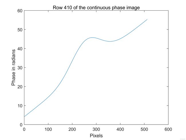
​ 我们会在下文介绍二维相位展开过程。假设我们有一个由计算机生成的且不包含任何相位包裹（2$\pi$跳变）的连续相位图像。该图像可显示为阵列图像，如图1(a)所示。相同的图像也由3D表面展示，如图1(b)所示。图像中一行（行410）的强度以图形方式在图1©中显示。生成此相位图像的matlab代码如下。Matlab函数peaks用于产生连续相位图像。请注意，我们这里用术语“连续”不是指模拟信号，而是指不含有任何相位包裹的离散一维相位信号或离散二维相位图像。

%这个程序是模拟一个连续相位分布来作为一个数据集用于二维相位展开问题中
clc; close all; clear
N = 512;
[x,y]=meshgrid(1:N);
image1 = 2*peaks(N) + 0.1*x + 0.01*y;
figure, colormap(gray(256)), imagesc(image1)
title('Continuous phase image displayed as a visual intensity array')
xlabel('Pixels'), ylabel('Pixels')
figure
surf(image1,'FaceColor','interp', 'EdgeColor','none', 'FaceLighting','phong')
view(-30,30), camlight left, axis tight
title(' Continuous phase map image displayed as a surface plot')
xlabel('Pixels'), ylabel('Pixels'), zlabel('Phase in radians')
figure, plot(image1(410,:))
title('Row 410 of the continuous phase image')
xlabel('Pixels'), ylabel('Phase in radians')

（a）

（b）

（c）

图1:(a)显示为视觉强度阵列的计算机生成连续相位图，(b)绘制为表面的相同图像，©相位图像中410行强度。

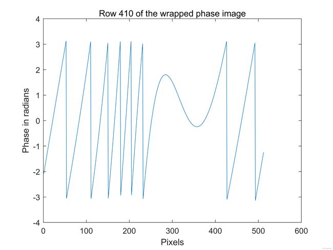
​ 现在让我们包裹计算机生成的连续相位图像。执行这个任务的Matlab代码如下：

%wrap the 2D image
image1_wrapped = atan2(sin(image1), cos(image1));
figure, colormap(gray(256)), imagesc(image1_wrapped)
title('Wrapped phase image displayed as a visual intensity array')
xlabel('Pixels'), ylabel('Pixels')
figure
surf(image1_wrapped,'FaceColor','interp', 'EdgeColor','none',
'FaceLighting','phong')
view(-30,70), camlight left, axis tight
title('Wrapped phase image plotted as a surface')
xlabel('Pixels'), ylabel('Pixels'), zlabel('Phase in radians')
figure, plot(image1_wrapped(410,:))
title('Row 410 of the wrapped phase image')
xlabel('Pixels'), ylabel('Phase in radians')

包裹后的图像如下所示：

（a）

（b）

（c）
图2:(a)显示为视觉强度阵列的一个包裹相位图，(b)绘制为表面的包裹图像，©包裹相位图中行410。

​ 回忆一维相位解缠绕辅导材料，当我们处理相位值线时，相位包裹显示为2$\pi$跳变，形成如图2©所示的锯齿波纹。注意在二维情况下，我们有二维数组形成的相位图，相位包裹显示为轮廓曲线，如图2(a)所示，我们也习惯称其为包裹曲线。这些曲线以闭合曲线、开放曲线和在图2(a)中两种共有形式存在。注意到后续案例中，如果一个开放曲线进入到一个包裹相位图，它一次必须分离。

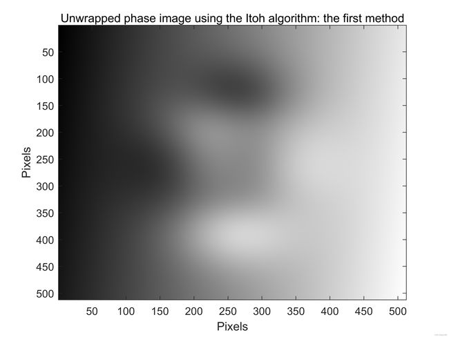
​ 为了展开图像，我们可以使用Itoh二维相位展开器。Itoh二维相位展开器主要由两种主要的方法可以实施。第一种方法包括在包裹图像中按行顺序展开（一次一个）。这会产生一个仅部分相位展开的中间图像。下面我们展示相似的过程，但是这次将部分解包裹图像中的所有列展开。由Itoh解包器第一个实现产生的相位解包图如图3(a)、(b)所示。执行此任务的Matlab代码如下所示：

%Unwrap the image using the Itoh algorithm: the second method
%performed by first sequentially unwrapping all the columns one at a time.
image2_unwrapped = image1_wrapped;
for i=1:N
image2_unwrapped(:,i) = unwrap(image2_unwrapped(:,i));
end
%Then sequentially unwrap all the a rows one at a time
for i=1:N
image2_unwrapped(i,:) = unwrap(image2_unwrapped(i,:));
end
figure, colormap(gray(256)), imagesc(image2_unwrapped)
title('Unwrapped phase image using Itoh algorithm: the second method')
xlabel('Pixels'), ylabel('Pixels')
figure
surf(image2_unwrapped,'FaceColor','interp', 'EdgeColor','none',
'FaceLighting','phong')
view(-30,30), camlight left, axis tight
title('Unwrapped phase image using the Itoh algorithm: the second method')
xlabel('Pixels'), ylabel('Pixels'), zlabel('Phase in radians')

​ 第二种实现Itoh解包器的方法恰好相反。换句话说，它首先设计一次一个解开包裹相位图中的所有列。并且这个也产生部分相位解包裹图。然后我们继续展开部分解包图像中的所有行。使用Itoh解包器的第二个实现产生的解包相位图如图3(b)所示。执行此任务的Matlab代码如下：

%Unwrap the image using the Itoh algorithm: the second method
%performed by first sequentially unwrapping all the columns one at a time.
image2_unwrapped = image1_wrapped;
for i=1:N
image2_unwrapped(:,i) = unwrap(image2_unwrapped(:,i));
end
%Then sequentially unwrap all the a rows one at a time
for i=1:N
image2_unwrapped(i,:) = unwrap(image2_unwrapped(i,:));
end
figure, colormap(gray(256)), imagesc(image2_unwrapped)
title('Unwrapped phase image using Itoh algorithm: the second method')
xlabel('Pixels'), ylabel('Pixels')
figure
surf(image2_unwrapped,'FaceColor','interp', 'EdgeColor','none',
'FaceLighting','phong')
view(-30,30), camlight left, axis tight
title('Unwrapped phase image using the Itoh algorithm: the second method')
xlabel('Pixels'), ylabel('Pixels'), zlabel('Phase in radians')

​ (a) (b)


​© (d)

图3：使用二维Itoh算法的解相图；(a)和(b)使用第一种方法；©和(d)使用第二种方法。

​ 从上面执行的练习中可以看出，两个Itoh相位解包裹算法的执行实际上创造了相同的输出结果。这是因为这个包裹相位图不是真实的，而是一个不包含任何误差的人造数据集。

​ 如图2(a)所示的包裹相位图是一个不包含任何误差源的理想相位图。我们可以使用二维相位解包器来处理这个图象。如上所述，这个例子我们使用二维Itoh算法畜栏里图像。这是一个非常简单的相位解包裹算法，它仅适用于没有相位误差的情况下。大多数实际应用程序都会产生包含误差的包裹相位图。在这个例子中，我们需要利用更多更复杂的二维相位解包裹器来处理这些图像。

​ 在二维相位展开中，四个误差源使得相位展开过程变得复杂。误差源如下所示：

​ 1、噪声

​ 2、采样不足

​ 3、当连续相位图包含突然、突变的相位变化

​ 4、相位提取算法自身产生的误差

​ 在本教程中，我们仅讨论前三个误差来源，并且它们对二维相位展开过程的影响。我们也会解释在这三个不同的情况下如何成功进行相位展开。第四个误差源取决于用于提取包裹相位的特定算法。读者应该意识到当运行相位展开时，会有其他潜在的误差源，但是关于算法本身对提取的包裹相位影响的详细讨论超出了本教程的范围，此处将不予介绍。

2、噪声对二维相位展开的影响

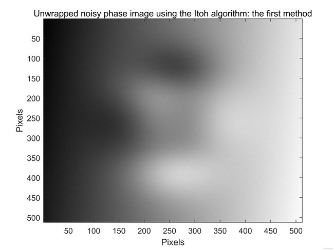
​ 相位展开器通过计算两个连续样本之间的差异来检测图像中是否存在相位包裹。如果这个差异超过$+\pi$，然后相位展开器认为这里有一个包裹值。这里可能是一个真正的相位包裹值，也有可能是一个由于噪声存在引起的假包裹值。为了研究噪声对二维相位展开的影响，让我们向之前展示的仿真的连续相位图1(a)中添加噪声，然后我们包裹噪声相位图。之后，我们尝试对模拟对象进行相位展开。这个过程在后续的Matlab程序实现。这里噪声的方差值为0.4。从图4中我们可以看出，如此低水平的噪声不会对Itoh展开算法产生不利的影响。

%This program shows the problems encountered when unwrapping a noisy 2D phase
%image by using computer simulation
clc; close all; clear
N = 512;
[x,y]=meshgrid(1:N);
noise_variance = 0.4;
image1 = 2*peaks(N) + 0.1*x + 0.01*y + noise_variance*randn(N,N);
figure, colormap(gray(256)), imagesc(image1)
title('Noisy continuous phase image displayed as visual intensity array')
xlabel('Pixels'), ylabel('Pixels')
figure
surf(image1,'FaceColor','interp', 'EdgeColor','none', 'FaceLighting','phong')
view(-30,30), camlight left, axis tight
title('Noisy continuous phase image displayed as a surface plot')
xlabel('Pixels'), ylabel('Pixels'), zlabel('Phase in radians')
figure, plot(image1(410,:))
title('Row 410 of the original noisy continuous phase image')
xlabel('Pixels'), ylabel('Phase in radians')
%wrap the 2D image
image1_wrapped = atan2(sin(image1), cos(image1));
figure, colormap(gray(256)), imagesc(image1_wrapped)
title('Noisy wrapped phase image displayed as visual intensity array')
xlabel('Pixels'), ylabel('Pixels')
figure
surf(image1_wrapped,'FaceColor','interp', 'EdgeColor','none','FaceLighting','phong')
view(-30,70), camlight left, axis tight
title('Noisy wrapped phase image plotted as a surface plot')
xlabel('Pixels'), ylabel('Pixels'), zlabel('Phase in radians')
figure, plot(image1_wrapped(410,:))
title('Row 410 of the wrapped noisy image')
xlabel('Pixels'), ylabel('Phase in radians')
%Unwrap the image using the Itoh algorithm: the first method
%Unwrap the image first by sequentially unwrapping the rows one at a time.
image1_unwrapped = image1_wrapped;
for i=1:N7
image1_unwrapped(i,:) = unwrap(image1_unwrapped(i,:));
end
%Then unwrap all the columns one-by-one
for i=1:N
image1_unwrapped(:,i) = unwrap(image1_unwrapped(:,i));
end
figure, colormap(gray(256)), imagesc(image1_unwrapped)
title('Unwrapped noisy phase image using the Itoh algorithm: the first method')
xlabel('Pixels'), ylabel('Pixels')
figure
surf(image1_unwrapped,'FaceColor','interp', 'EdgeColor','none','FaceLighting','phong')
view(-30,30), camlight left, axis tight
title('Unwrapped noisy phase image using the Itoh unwrapper: the first method')
xlabel('Pixels'), ylabel('Pixels'), zlabel('Phase in radians')
%Unwrap the image using the Itoh algorithm: the second method
%Unwrap the image by first sequentially unwrapping all the columns.
image2_unwrapped = image1_wrapped;
for i=1:N
image2_unwrapped(:,i) = unwrap(image2_unwrapped(:,i));
end
%Then unwrap all the a rows one-by-one
for i=1:N
image2_unwrapped(i,:) = unwrap(image2_unwrapped(i,:));
end
figure, colormap(gray(256)), imagesc(image2_unwrapped)
title('Unwrapped noisy image using the Itoh algorithm: the second method')
xlabel('Pixels'), ylabel('Pixels')
figure
surf(image2_unwrapped,'FaceColor','interp', 'EdgeColor','none','FaceLighting','phong')
view(-30,30), camlight left, axis tight
title('Unwrapped noisy phase image using the Itoh algorithm: the second method')
xlabel('Pixels'), ylabel('Pixels'), zlabel('Phase in radians')

​ (a) (b)

© (d)

(e) (f)

(g) (h)

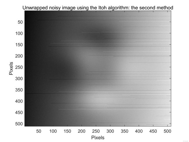
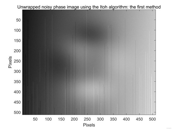
图4：(a)和(b)计算机生成的噪声连续相位图。©和(d)包裹的噪声相位图。(e)和(f)使用Itoh算法第一种方法的相位展开图。(g)和(h)是哦弄个Itoh算法第二种方法的相位展开图。此处噪声方差为0.4。

%This program shows the problems encountered when unwrapping a noisy 2D phase
%image by using computer simulation
clc; close all; clear
N = 512;
[x,y]=meshgrid(1:N);
noise_variance = 0.4;
image1 = 2*peaks(N) + 0.1*x + 0.01*y + noise_variance*randn(N,N);
figure, colormap(gray(256)), imagesc(image1)
title('Noisy continuous phase image displayed as visual intensity array')
xlabel('Pixels'), ylabel('Pixels')
figure
surf(image1,'FaceColor','interp', 'EdgeColor','none', 'FaceLighting','phong')
view(-30,30), camlight left, axis tight
title('Noisy continuous phase image displayed as a surface plot')
xlabel('Pixels'), ylabel('Pixels'), zlabel('Phase in radians')
figure, plot(image1(410,:))
title('Row 410 of the original noisy continuous phase image')
xlabel('Pixels'), ylabel('Phase in radians')
%wrap the 2D image
image1_wrapped = atan2(sin(image1), cos(image1));
figure, colormap(gray(256)), imagesc(image1_wrapped)
title('Noisy wrapped phase image displayed as visual intensity array')
xlabel('Pixels'), ylabel('Pixels')
figure
surf(image1_wrapped,'FaceColor','interp', 'EdgeColor','none','FaceLighting','phong')
view(-30,70), camlight left, axis tight
title('Noisy wrapped phase image plotted as a surface plot')
xlabel('Pixels'), ylabel('Pixels'), zlabel('Phase in radians')
figure, plot(image1_wrapped(410,:))
title('Row 410 of the wrapped noisy image')
xlabel('Pixels'), ylabel('Phase in radians')
%Unwrap the image using the Itoh algorithm: the first method
%Unwrap the image first by sequentially unwrapping the rows one at a time.
image1_unwrapped = image1_wrapped;
for i=1:N7
image1_unwrapped(i,:) = unwrap(image1_unwrapped(i,:));
end
%Then unwrap all the columns one-by-one
for i=1:N
image1_unwrapped(:,i) = unwrap(image1_unwrapped(:,i));
end
figure, colormap(gray(256)), imagesc(image1_unwrapped)
title('Unwrapped noisy phase image using the Itoh algorithm: the first method')
xlabel('Pixels'), ylabel('Pixels')
figure
surf(image1_unwrapped,'FaceColor','interp', 'EdgeColor','none','FaceLighting','phong')
view(-30,30), camlight left, axis tight
title('Unwrapped noisy phase image using the Itoh unwrapper: the first method')
xlabel('Pixels'), ylabel('Pixels'), zlabel('Phase in radians')
%Unwrap the image using the Itoh algorithm: the second method
%Unwrap the image by first sequentially unwrapping all the columns.
image2_unwrapped = image1_wrapped;
for i=1:N
image2_unwrapped(:,i) = unwrap(image2_unwrapped(:,i));
end
%Then unwrap all the a rows one-by-one
for i=1:N
image2_unwrapped(i,:) = unwrap(image2_unwrapped(i,:));
end
figure, colormap(gray(256)), imagesc(image2_unwrapped)
title('Unwrapped noisy image using the Itoh algorithm: the second method')
xlabel('Pixels'), ylabel('Pixels')
figure
surf(image2_unwrapped,'FaceColor','interp', 'EdgeColor','none','FaceLighting','phong')
view(-30,30), camlight left, axis tight
title('Unwrapped noisy phase image using the Itoh algorithm: the second method')
xlabel('Pixels'), ylabel('Pixels'), zlabel('Phase in radians')

(a) (b)


（c） （d）


（e） （f）


（g） （h)

图5：(a)和(b)计算机生成的噪声连续相位图。©和(d)包裹的噪声相位图。(e)和(f)使用Itoh算法第一种方法的相位展开图。(g)和(h)是哦弄个Itoh算法第二种方法的相位展开图。此处噪声方差为0.6。

​ 当我们将噪声方差增加到0.6时便会出现问题。在这种情况下，Itoh相位展开算法无法成功展开图像。注意到展开相位图中任然存在$2\pi$不连续性。还要注意，执行Itoh算法的第一种和第二种方法产生了不同的结果。

​ 正如一维相位展开教程中所提到的，在相位展开过程中会出现误差积累，并且这就使得含噪声的二维包裹相位图展开过程复杂化。图5(e)展示了一张使用第一种Itoh算法处理的图像。这个算法首先依次展开所有行，当所有行全部展开完成后，它随后会继续逐次展开所有列。仔细检查图5(e)可以发现许多关于误差积累问题的信息。例如，在图5(e)中行455包含假包裹。这个假包裹会产生一个$2\pi$误差，这个误差会在整行中传播，从假包裹的位置一直到行尾。相似的误差也在处理这个包裹相位图中许多其他行中出现。使用第一种Itoh相位解包裹算法实现，$2\pi$误差处在结果相位图中显示为水平线。

​ 图5(g)显示了执行第二种Itoh算法方法的过程。相较于第一实现相比，这个算法改变了展开行和列的相位顺序。换句话说，它首先依次展开图像中的所有列，然后，当展开所有列后，算法依次展开所有行。仔细观察图5(g)可以看出可以看出关于误差积累问题的一些信息。例如，图5(g)列360包含了一个假包裹。这个假包裹会产生一个$2\pi$误差，这个误差会在整列中传播，从假包裹的位置一直到列尾。相似的误差也在处理这个包裹相位图中许多其他行中出现。使用第二种Itoh相位解包裹算法实现，$2\pi$误差处在结果相位图中显示为垂直线。

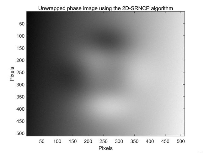
研究院已经发展了许多相位展开算法，来尝试阻止误差传播的发生。[2]中解释了其中一些算法。同样的，在LJMU中的综合工程研究所(General Engineering Research Institute, GERI)我们研发了一个名为2D-SRNCP phase unwrapper自动二维相位展开算法[3]。我们算法是基于可靠性排序，跟随非连续路径，并且在处理含有噪声破坏的真实包裹相位图中表现出了出色的表现，不需要关心它如何工作的细节，只需要将它作为一个非常先进和鲁棒的展开算法并将它作为工具去使用。你们可以通过网址http://www.ljmu.ac.uk/GERI/90225.htm在Matlab中下载2D-SRNCP相位展开器。

​ 图5©中的包裹相位图时使用2D-SRNCP相位展开器生成的。相关图像显示为图6©视觉强度阵列和图6(d)3D表面。对比图6©和(d)与图5©和(d)可以看出，我们的算法成功地正确处理了包裹相位图并防止了误差的传播。

​ 请注意2D-SRNCP phase unwrap 是用C语言编写的。这个C程序可以使用Mex ’Matlab Executable’ 动态链接子程序功能从Matlab调用。这个C代码在调用前要先在Matlab中编译。在Matlab中编译C代码，在Matlab提示框中键入以下代码：mex Miguel_2D_unwrapper.cpp

​ 下面给出了用于展开图像的matlab代码：

%How to call the 2D-SRNCP phase unwrapper from the C language
%You should have already compiled the phase unwrapper’s C code first
%If you haven’t, to compile the C code: in the Matlab Command Window type
% mex Miguel_2D_unwrapper.cpp
%The wrapped phase that you present as an input to the compiled C function
%should have the single data type (float in C)
WrappedPhase = double(image1_wrapped);
UnwrappedPhase = Miguel_2D_unwrapper(WrappedPhase);
figure, colormap(gray(256))
imagesc(UnwrappedPhase);
xlabel('Pixels'), ylabel('Pixels')
title('Unwrapped phase image using the 2D-SRNCP algorithm')
figure
surf(double(UnwrappedPhase),'FaceColor','interp', 'EdgeColor','none','FaceLighting','phong')
view(-30,30), camlight left, axis tight
title('Unwrapped phase image using the 2D-SRNCP displayed as a surface')
xlabel('Pixels'), ylabel('Pixels'), zlabel('Phase in radians')

（a） （b）

图6：(a)和(b)使用2D-SRNCP的展开相位

---

3、欠采样对二维相位展开的影响

正如之前所介绍的，相位展开器通过检测两幅连续样本之间的差异来判断是否有包裹。如果这个差异值大于$+\pi$或者小于$-\pi$，则相位展开器认为此处有一个包裹。这里可能是一个真实包裹相位，也可能是一个由噪声或者欠采样造成的假包裹。

欠采样相位图像的相位展开是困难的，甚至一些情况下是不可能的。当两个连续样本的差异大于$+\pi$或者小于$-\pi$时就会发生。两个毗邻样本大的差别的出现仅由于相位图没有包含足够的样本，而不是由于真实相位包裹的存在。这种情况会自动生成不正确的假包裹。

让我们首先回顾一维相位展开过程中欠采样的影响。根据奈奎斯特采样定律，如果一个函数$f(x)$不包含高于$B$赫兹的频率，则可以通过$2B$或者更高频率的采样完全确定它。在$f(x)$是完全正弦信号的情况下，$f(x)$的每一个周期必须由至少两个样本来采样。这个原则也适用于包裹相位信号中。

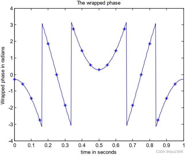
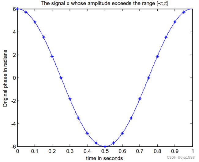
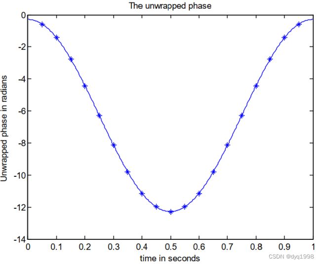
假设我们考虑如图7(a)所示的一维连续相位信号。这个信号包含20个样本，正好覆盖循环波形的一个周期。这个信号的相位包裹如图7(b)所示。这个包裹信号由足够高频率的信号采样，并且它包含四个完整包裹。这个包裹信号肯能使用一维Itoh算法进行相位展开，展开结果如图7©所示。注意到这种情况下相对简单的1D Itoh算法正确地展开了包裹相位信号。同时也注意到尽管展开信号的形状跟原始信号是相同的，图表中每个点的真实相位值是不同的，例如，图7(a)中原始信号的范围是从$+6$到$-6$弧度，而图7©中展开信号的范围是从0到$-12$弧度。同时也应该注意到大多数相位展开的输出仅仅产生如此”相似“而非”绝对“相位值。每此代码运行，许多先进的展开器会产生相同形状的相似相位输出，但绝对相位值的数字不同。应该注意到，可以采用某些实际测量绝对相位而不是相对相位的测量策略。

（a） （b） （c）

图7：（a）一个包含20个样本的连续相位信号。（b）相位包裹信号。（c）相位展开信号。

​

现在让我们减少与图7（a）中相同1D相位信号的样本数量，将采样频率减半，这样这个信号仅有10个样本，如图8(a)所示。然后如图8(b)所示将这个信号展开。这个包裹信号现在包含四个完整包裹和两个假包裹。信号欠采样率导致了两个假包裹的出现，它们的位置在图8(b)中高亮标出。第三和第四样本之间的差异小于$-\pi$。一个相位展开器会将这种大的差异当成一个包裹，并且将会向第四个样本及它右侧所有的样本增加$2\pi$，如图8©所示。这会破坏整个一维相位展开信号。同样的，第八和第九个样本之间的差异大于$+\pi$，相位展开器有一次认为这里是一个包裹，并且因此从第九和第十样本减去$2\pi$，如图8©所示。这同样会破坏1D相位展开信号。注意到展开相位信号现在已经与如图8(a)所示的原始连续相位信号完全不同了。请注意，此处使用了1D Itoh算法处理了此信号。

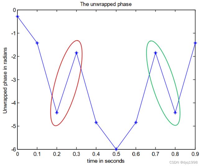
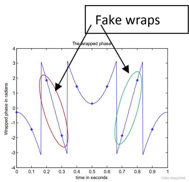
图8：（a）现在仅包含10个采样点的连续相位信号。（b）包裹信号。（c）展开信号。

接下来我们将通过电脑模拟的欠采样相位图来解释欠采样对2D相位展开算法的影响。首先我们制造人工欠采样相位图。然后我们根据采样定律理论分析电脑生成的相位图，以研究对特殊数据集在$x$和$y$方向上的最大允许采样率。下面我们将包裹这些图像。之后我们使用两种不同的相位展开算法来处理图像，即Itoh算法和2D-SRNCP算法。最后我们将这两种展开算法处理的图像与原始线序相位图做对比。

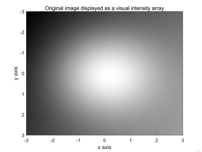
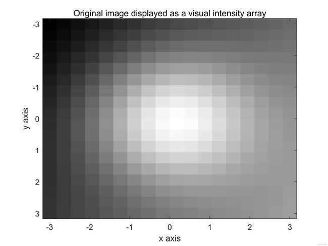
假设我们有由计算机产生的连续相位图$f(x,y)$，在图中既显示为图9(a)视觉强度阵列，又显示为图9(b)中3D表面相位图，并由如下公式表示：
$$f(x,y)=20e^{-\frac{1}{4}(x^2+y^2)}+2x+y,-3\le x\le 3,-3\le y\le 3$$
现在我们根据采样定律分析这个仿真相位图。

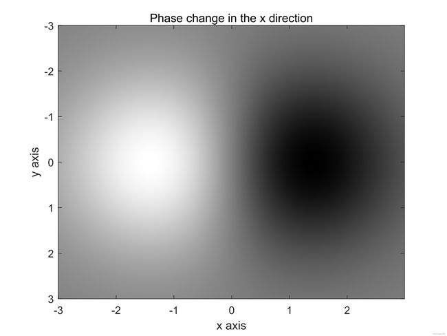
首先让我们找到这个数据集中$x$方向上最大的相位变化率。相位图象上$x$方向的相位变化率如图9©所示，由下面公式给出，该公式由上述公式对$x$求偏微分得出；
$$\frac{\partial f(x,y)}{\partial x}=-10x{e}^{\frac{1}{4}(x^2+y^2)}+2$$
$x$方向上的最大相位变化的实际位置出现在此连续相位图像$x=-1.4172$和$y=-0.0015$处。此处的最大相位变化值为10.5776弧度。

因此，如果$x$方向的连续样本必须改变一个小于$\pi$的值，以便它们不会被错误地标记为包裹，然后采样率（一个周期的样本数，表示为$N_x$）由如下公式给出：
$$N_x>\frac{10.5776}{\pi }=3.367$$
此示例方程在$x$方向上采样的实际数据点数$N_{Rx}$由如下公式给出：
$$N_{Rx}=R_x{N}_x$$
其中$N_x$是$x$方向的采样率，$R_x$是$x$方向的数据范围，对于此处给出的示例范围为$R_x=6(6--3)$。

然后，根据上式：
$$N_{Rx}=6.0\times 3.367=20.2020$$
因此，这里生成的连续相位图像在$x$方向上至少采样21个样本，否则就会欠采样。如果在$x$方向上的采样少于21个采样点，然后这样的欠采样会导致两个连续样本之间的差异大于$\pi$，这会在使用展开算法处理时错误在该处产生假包裹。

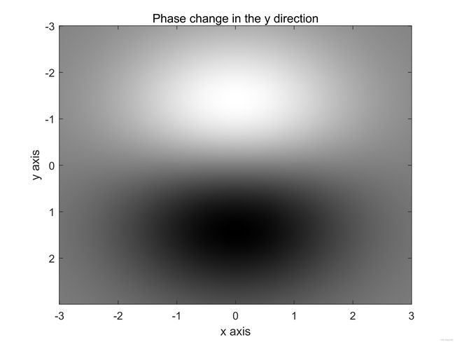
类似地，在图9(d)中展示了$y$方向的相位变化率，并由以下公式给出，该公式由本节开始时介绍的公式$f(x,y)$进行偏微分运算得出，这次是关于$y$方向的：
$$\frac{\partial f(x,y)}{\partial y}=-10y{e}^{-\frac{1}{4}(x^2+y^2)}+1$$
在这个连续相位图中$y$方向上最大相位变化出现在点$x=-0.0044$和$y=-1.4143$位置处。此处$y$方向上最大相位变化值为9.5776弧度。

因此，如果$y$方向上连续样本必须变化一个小于$\pi$的值，以便它们不会被错误地标记为包裹，采样率（一个周期样本数，表示为$N_y$）由如下公式给出：
$$N_y>\frac{9.5776}{\pi }=3.0486$$
对此例子$N_{Ry}$上$y$方向采样的实际数据点数目有下面公式给出：
$$N_{Ry}=R_y{N}_y$$
其中$N_y$是$y$方向的采样率，$R_y$是$y$像素的数据范围，此例的范围为$R_y=6(6=3--3)$

然后，根据如下公式：
$$N_{Ry}=6.0\times 3.0486=18.2916$$
因此，这里生成的连续相位图在$y$方向上必须采样至少19个样本，防止欠采样和假包裹错误的生成。

下面给出了创建和绘制此模拟连续相位数据集的代码，以及相位$x$和$y$的变化率。

clc; close all; clear
NRx = 512; NRy=512;
tx = linspace(-3,3,NRx);
ty = linspace(-3,3,NRy);
[x,y]=meshgrid(tx,ty);
image1 = 20*exp(-0.25*(x.^2 + y.^2)) + 2*x + y;
figure, colormap(gray(256)), imagesc(tx,ty,image1)
title('Original image displayed as a visual intensity array')
xlabel('x axis'), ylabel('y axis')
figure
surf(x,y,image1,'FaceColor','interp', 'EdgeColor','none','FaceLighting','phong')
view(-30,30), camlight left, axis tight
title('Original image displayed as a surface plot')
xlabel('x axis'), ylabel('y axis'), zlabel('Phase in radians')
xdiff = diff(image1')';
figure, colormap(gray(256)), imagesc(tx(1:end-1),ty,xdiff)
title('Phase change in the x direction')
xlabel('x axis'), ylabel('y axis')
ydiff = diff(image1);
figure, colormap(gray(256)), imagesc(tx,ty(1:end-1),ydiff)
title('Phase change in the y direction')
xlabel('x axis'), ylabel('y axis')

​ (a) (b)

​ © (d)

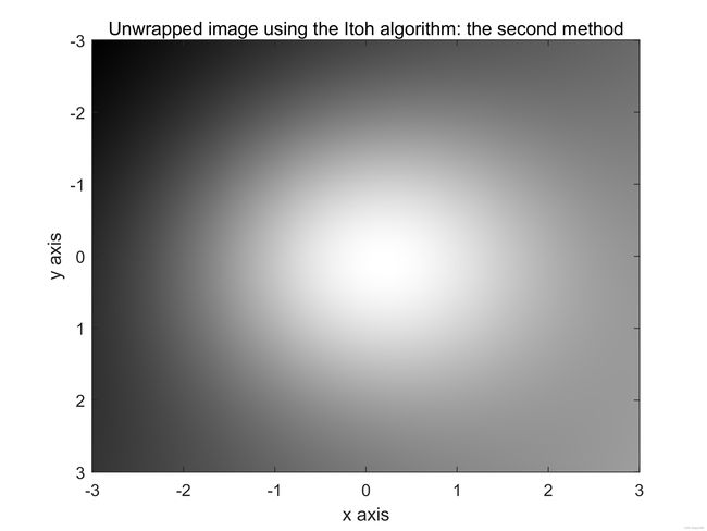
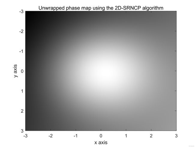
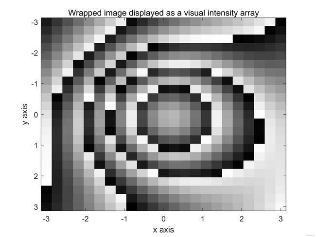
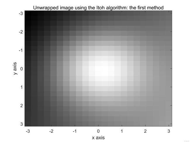
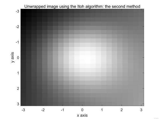
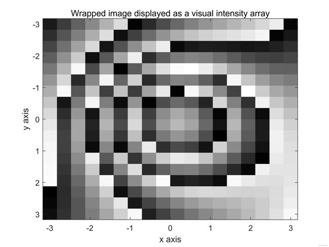
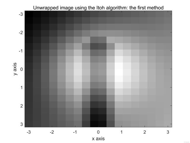
图9：(a)和(b)一个计算机生成的连续相位图。©和(d)计算机生成连续相位图分别在$x$和$y$方向的两位变化。此处，$N_{Rx}=512$，$N_{Ry}=512$。继续…

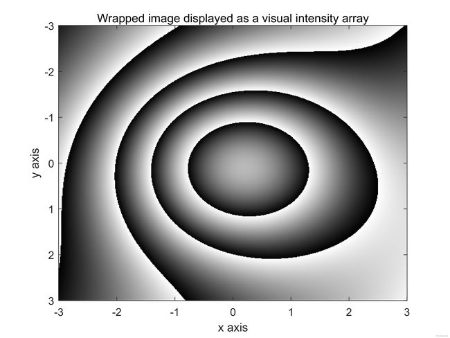
计算机生成的连续相位图仙子啊可以人工包裹，其结果如图9(e)和(f)所示。使用Itoh算法的第一种方法展开包裹相位图像。如图9(g)和(h)所示。下面使用Itoh算法的第二种方法展开包裹相位图像，其结果如图9(i)和(j)所示，最后，使用2D-SRNCP算法展开包裹相位图，其结果如图9(k)和(l)所示。

​ (e) (f)

​ (g) (h)

​ (i) (j)

​ (k) (l)

图9：续。(e)和(f)包裹图像。图(g)和(h)使用Itoh算法的第一种方法进行处理，图(i)和(j)使用Itoh算法第二种方法处理，图(k)和(l)使用2D-SRNCP算法处理。此处，采样率很高，$N_{Rx}=512$和$N_{Ry}=512$。

下面给出了用于生成图9所示的所有图像的Matlab代码。这里$N_{Rx}$的值设置为512，相应的$N_{Ry}$的值也设置为512.注意到三个相位展开算法都成功的展开了包裹相位图，如图9(e)所示。

%wrap the 2D image
image1_wrapped = atan2(sin(image1), cos(image1));
figure, colormap(gray(256)), imagesc(tx,ty,image1_wrapped)
title('Wrapped image displayed as a visual intensity array')
xlabel('x axis'), ylabel('y axis')
figure
surf(x,y,image1_wrapped,'FaceColor','interp', 'EdgeColor','none','FaceLighting','phong')
view(-30,70), camlight left, axis tight
title('Wrapped image plotted as a surface')
xlabel('x axis'), ylabel('y axis'), zlabel('Phase in radians')
%Unwrap the image using the Itoh algorithm: implemented using the first method
%Unwrap the image by firstly unwrapping all the rows, one at a time.
image1_unwrapped = image1_wrapped;
for i=1:NRy
image1_unwrapped(i,:) = unwrap(image1_unwrapped(i,:));
end
%Then unwrap all the columns, one at a time
for i=1:NRx
image1_unwrapped(:,i) = unwrap(image1_unwrapped(:,i));
end
figure, colormap(gray(256)), imagesc(tx,ty,image1_unwrapped)
title('Unwrapped image using the Itoh algorithm: the first method')
xlabel('x axis'), ylabel('y axis')
figure
surf(x,y,image1_unwrapped,'FaceColor','interp', 'EdgeColor','none','FaceLighting','phong')
view(-30,30), camlight left, axis tight
title('Unwrapped phase map using the Itoh unwrapper: the first method')
xlabel('x axis'), ylabel('y axis'), zlabel('Phase in radians')
%Unwrap the image using the Itoh algorithm: implemented using the second method
%Unwrap the image by firstly unwrapping all the columns one at a time.
image2_unwrapped = image1_wrapped;
for i=1:NRx
image2_unwrapped(:,i) = unwrap(image2_unwrapped(:,i));
end
%Then unwrap all the a rows one at a time
for i=1:NRy
image2_unwrapped(i,:) = unwrap(image2_unwrapped(i,:));
end
figure, colormap(gray(256)), imagesc(tx,ty,image2_unwrapped)
title('Unwrapped image using the Itoh algorithm: the second method')
xlabel('x axis'), ylabel('y axis')
figure
surf(x,y,image2_unwrapped,'FaceColor','interp', 'EdgeColor','none','FaceLighting','phong')
view(-30,30), camlight left, axis tight
title('Unwrapped phase map using the Itoh algorithm: the second method')
xlabel('x axis'), ylabel('y axis'), zlabel('Phase in radians')
%call the 2D phase unwrapper from the C language
%To compile the C code: in Matlab Command Window type
% mex Miguel_2D_unwrapper.cpp
%The wrapped phase should have the double data type (float in C)
WrappedPhase = double(image1_wrapped);
UnwrappedPhase = Miguel_2D_unwrapper(WrappedPhase);
figure, colormap(gray(256))
imagesc(tx,ty,UnwrappedPhase);
xlabel('x axis'), ylabel('y axis')
title('Unwrapped phase map using the 2D-SRNCP algorithm')
figure
surf(x,y,double(UnwrappedPhase),'FaceColor','interp', 'EdgeColor','none','FaceLighting','phong')
view(-30,30), camlight left, axis tight
title('Unwrapped phase map using the 2D-SRNCP displayed as a surface plot')
xlabel('x axis'), ylabel('y axis'), zlabel('Phase in radians')

上述算法现在重复一遍，但这次降低了采样率，$N_{Rx}$的值设置为23，$N_{Ry}$的值设置为21。从结果可以看出所有的相位展开算法都成功的展开了包裹的相位图像，如图10©所示。得到的相位展开图像如图10所示。

​ (a) (b)

​ © (d)

​ (e) (f)

​ (g) (h)

​ (i) (j)

图10：(a)和(b)计算机生成的连续相位图。©和(d)包裹图像。(e)和(f)使用Itoh算法第一种方法展开的图像。(g)和(h)使用Itoh算法第二种方法展开的图像。(i)和(j)使用2D-SRNCP算法展开的图像。此处降低了采样率，但也仍高于理论最小值允许限制，$N_{Rx}=23,N_{Ry}=23$。

现在再次重复上述过程，但现在将$N_{Rx}$设置为20，$N_{Ry}$设置为20（即低于理论最小采样率）。通过将$N_{Rx}$和$N_{Ry}$设置为这些值，计算机生成的连续相位图像现处于欠采样状态。从图11(e)-(h)中可以看出，Itoh算法未能成功的展开包裹的相位图像。在这里，由欠采样引起的假包裹产生错误会在整个图像中传播。另一方面，2D-SRNCP相位展开器虽然不能防止错误的发生，并且错误明显存在于展开的相位图中，但确实可以防止这样的错误在图像中传播并破坏好的数据，如图11(i)和(j)所示。

​ (a) (b)

​ © (d)

​ (e) (f)

​ (g) (h)

​ (i) (j)

图11：(a)和(b)计算机生成的连续相位图。©和(d)包裹图像。(e)和(f)使用Itoh算法第一种方法展开的图像。(g)和(h)使用Itoh算法第二种方法展开的图像。(i)和(j)使用2D-SRNCP算法展开的图像。此处降低了采样率，但也仍高于理论最小值允许限制，$N_{Rx}=18,N_{Ry}=18$。

4、相位不连续对二维相位展开的影响

包含突变的连续相位的相位展开是困难的，甚至是不可能的。这种情况出现在相位变化大于$+\pi$或者小于$-\pi$的时候。如此巨大而突然的相位变化可能被认为是真正的包裹，而实际上仅仅是由于突然的相位变化而存在的假包裹。或者，它们也可能会掩盖真实的相位包裹，导致它们消失。我们将在这里使用计算机生成相位图像来解释这些相位不连续对2D相位展开算法的影响。然后我们将包裹这些图像，之后我们将使用两种不同的算法来处理这些图像：即Itoh和2D-SRNCP算法。最后，我们将对比这些解包器生成的图像与原始连续相位图像进行比较。

4.1 示例1

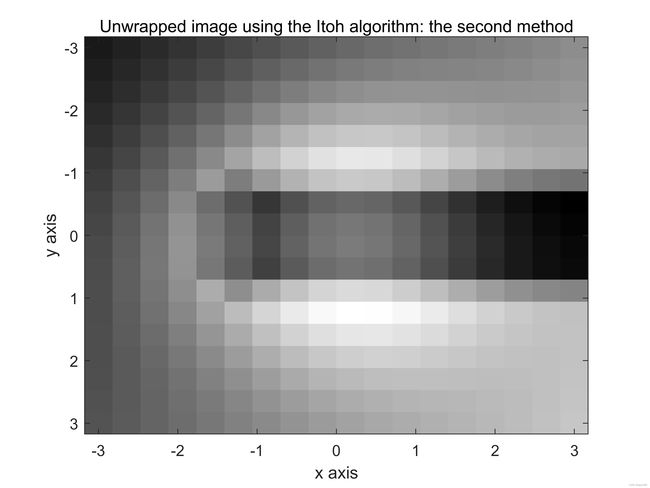
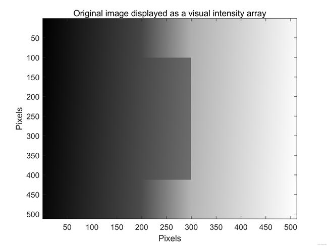
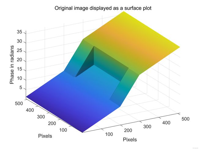
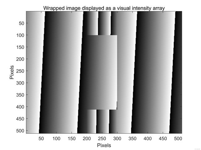
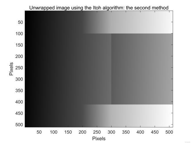
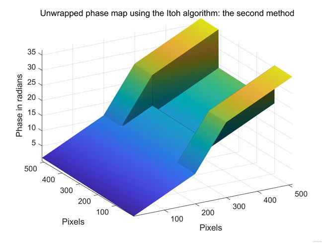
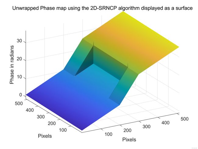
假设我们有计算机生成的连续相位图像，在图12(a)和10(b)中显示为视觉强度阵列和表面图。这些包含从100行到412行以及从第200列到第300列（含）的矩形区域内其相位的突然变化。突变的相位变化幅度为10弧度。该相位图的Matlab实现显示在下面给出的Matlab代码中。

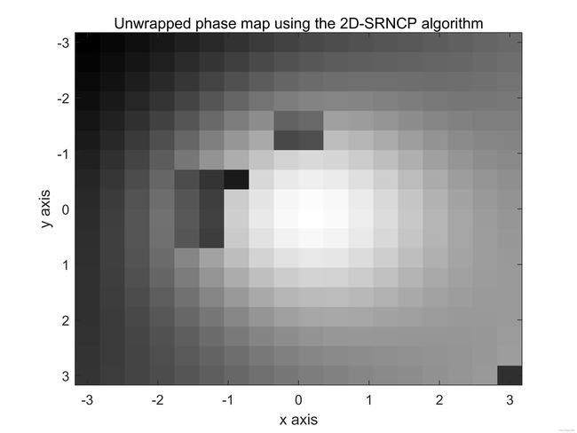
相位图像首先被包裹，然后使用之前提到的两种不同的相位展开算法进行展开。检查图12可以推断，Itoh算法没能成功的展开图像，2D-SRNCP算法成功展开了此相位图像。

仔细检查图12©会发现存在许多假包裹。例如，从第100行和第412行中存在许多假包裹。这些假包裹破坏了Itoh算法的正确操作：第一种方法，如图12(f)所示。非常多的假包裹（实际上由312个！）位于第300列。这些假包裹是由于在该位置发生的突然的5弧度的相位突变而产生的。这些假包裹破坏了Itoh算法的操作：第二种方法，如图12(h)所示。

​ (a) (b)

​ © (d)

​ (e) (f)

​ (g) (h)

​ (i) (j)

图12：(a)和(b)计算机生成的相位图。©和(d)包裹相位图。(e)和(f)使用Itoh算法第一种方法处理的相位展开图。(g)和(h)使用Itoh算法第二种方法处理的相位展开图。(i)和(j)使用2D-SRNCP算法处理的相位展开图。

用于生成图12图像的matlab代码由下面给出：

%This program is to simulate the 2D phase unwrapping problem
clc; close all; clear
N = 512;
[x,y] = meshgrid(1:N);
shape = zeros(N,N);
phaseChange = 10;
shape(:,300:end) = phaseChange;
x1=meshgrid(1:100);
shape(1:100,200:299) = x1*phaseChange/100;
shape(413:512,200:299) = x1*phaseChange/100;
image1 = shape + 0.05*x + 0.002*y;
figure, colormap(gray(256)), imagesc(image1)
title('Original image displayed as a visual intensity array')
xlabel('Pixels'), ylabel('Pixels')
figure
surf(image1,'FaceColor','interp', 'EdgeColor','none', 'FaceLighting','phong')
view(-30,30), camlight left, axis tight
title('Original image displayed as a surface plot')
xlabel('Pixels'), ylabel('Pixels'), zlabel('Phase in radians')
%wrap the 2D image
image1_wrapped = atan2(sin(image1), cos(image1));
figure, colormap(gray(256)), imagesc(image1_wrapped)
title('Wrapped image displayed as a visual intensity array')
xlabel('Pixels'), ylabel('Pixels')
figure
surf(image1_wrapped,'FaceColor','interp', 'EdgeColor','none','FaceLighting','phong')
view(-30,70), camlight left, axis tight
title('Wrapped image plotted as a surface plot')
xlabel('Pixels'), ylabel('Pixels'), zlabel('Phase in radians')
%Unwrap the image using Itoh the algorithm: the first method
%Unwrap the image by firstly unwrapping the rows one at a time.
image1_unwrapped = image1_wrapped;
for i=1:N
image1_unwrapped(i,:) = unwrap(image1_unwrapped(i,:));
end
%Then unwrap all the columns one at a time
for i=1:N
image1_unwrapped(:,i) = unwrap(image1_unwrapped(:,i));
end
figure, colormap(gray(256)), imagesc(image1_unwrapped)
title('Unwrapped image using the Itoh algorithm: the first method')
xlabel('Pixels'), ylabel('Pixels')
figure
surf(image1_unwrapped,'FaceColor','interp', 'EdgeColor','none','FaceLighting','phong')
view(-30,30), camlight left, axis tight
title('Unwrapped phase map using the Itoh unwrapper: the first method')
xlabel('Pixels'), ylabel('Pixels'), zlabel('Phase in radians')
%Unwrap the image using the Itoh algorithm: the second method
%Unwrap the image by firstly unwrapping all the columns one at a time.
image2_unwrapped = image1_wrapped;
for i=1:N
image2_unwrapped(:,i) = unwrap(image2_unwrapped(:,i));
end
%Then unwrap all the a rows one at a time
for i=1:N
image2_unwrapped(i,:) = unwrap(image2_unwrapped(i,:));
end
figure, colormap(gray(256)), imagesc(image2_unwrapped)
title('Unwrapped image using the Itoh algorithm: the second method')
xlabel('Pixels'), ylabel('Pixels')
figure
surf(image2_unwrapped,'FaceColor','interp', 'EdgeColor','none','FaceLighting','phong')
view(-30,30), camlight left, axis tight
title('Unwrapped phase map using the Itoh algorithm: the second method')
xlabel('Pixels'), ylabel('Pixels'), zlabel('Phase in radians')
%Call the 2D-SRNCP phase unwrapper from the C language code
%To compile the C code: in Matlab Command Window type
% mex Miguel_2D_unwrapper.cpp
%The wrapped phase should have the double data type (float in C)
WrappedPhase = double(image1_wrapped);
UnwrappedPhase = Miguel_2D_unwrapper(WrappedPhase);
figure, colormap(gray(256))
imagesc(UnwrappedPhase);
xlabel('Pixels'), ylabel('Pixels')
title('Unwrapped phase map using the 2D-SRNCP algorithm')
figure
surf(double(UnwrappedPhase),'FaceColor','interp', 'EdgeColor','none','FaceLighting','phong')
view(-30,30), camlight left, axis tight
title('Unwrapped Phase map using the 2D-SRNCP algorithm displayed as a surface')
xlabel('Pixels'), ylabel('Pixels'), zlabel('Phase in radians')

5、结论

提示：这里对文章进行总结：

以足够高的采样率采样并且不包含噪声或突然的相位变化的图像的相位展开先对简单，并且可以使用2D Itoh相位展开算法来执行该过程。然而，一旦这三个条件中的任何一个被违反，相位展开就会成为一项非常难以完成的任务。这是因为错误传播使得处理包裹相位图像中的一个像素的错误会影响图像中的其他像素。一个包裹相位图可能包含成十万甚至百万像素。一个相位展开算法成功处理单个像素可能造成图像中所有相位信息不可用。这使得二维相位展开过程很难正确执行。