机器学习---SVM一些简单的例子（XOR逻辑分类、最大间隔超平面、一维回归、SVM分类、权重、类别不平衡、核函数、单变量特征选择、参数C、非线性核、不同类型的SVM、正则化参数、RBF核参数组合）

1. XOR逻辑分类

        利用非线性支持向量机进行XOR逻辑的二元分类，并将决策函数在输入空间上的分布情况可

视化展示出来。

import numpy as np
import matplotlib.pyplot as plt
from sklearn import svm

xx, yy = np.meshgrid(np.linspace(-3, 3, 500),
                     np.linspace(-3, 3, 500))
np.random.seed(0)
X = np.random.randn(300, 2)
Y = np.logical_xor(X[:, 0] > 0, X[:, 1] > 0)

# fit the model
clf = svm.NuSVC()
clf.fit(X, Y)

# plot the decision function for each datapoint on the grid
Z = clf.decision_function(np.c_[xx.ravel(), yy.ravel()])
Z = Z.reshape(xx.shape)

plt.imshow(Z, interpolation='nearest',
           extent=(xx.min(), xx.max(), yy.min(), yy.max()), aspect='auto',
           origin='lower', cmap=plt.cm.PuOr_r)
contours = plt.contour(xx, yy, Z, levels=[0], linewidths=2,
                       linetypes='--')
plt.scatter(X[:, 0], X[:, 1], s=30, c=Y, cmap=plt.cm.Paired,
            edgecolors='k')
plt.xticks(())
plt.yticks(())
plt.axis([-3, 3, -3, 3])
plt.show()

np.meshgrid 生成一个网格，在 x 和 y 轴上均匀分布的点，用于创建输入空间。

使用 np.random.randn 生成300个二维的随机样本点。

Y 是基于这些样本点生成的XOR逻辑运算的结果。

创建一个支持向量机模型 clf，svm.NuSVC()是一种基于支持向量机的分类器。

计算决策函数在输入空间上的取值，并将其绘制成图像。

通过 clf.decision_function() 计算决策函数值。 

使用 plt.imshow() 将决策函数的取值以颜色的形式显示在图像上，用不同颜色表示不同决策区域。

plt.contour() 画出决策边界，使用虚线表示。

plt.scatter() 显示训练样本点，颜色由 Y 决定。 

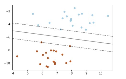
2. 最大间隔超平面

import numpy as np
import matplotlib.pyplot as plt
from sklearn import svm
from sklearn.datasets import make_blobs


# we create 40 separable points
X, y = make_blobs(n_samples=40, centers=2, random_state=6)

# fit the model, don't regularize for illustration purposes
clf = svm.SVC(kernel='linear', C=1000)
clf.fit(X, y)

plt.scatter(X[:, 0], X[:, 1], c=y, s=30, cmap=plt.cm.Paired)

# plot the decision function
ax = plt.gca()
xlim = ax.get_xlim()
ylim = ax.get_ylim()

# create grid to evaluate model
xx = np.linspace(xlim[0], xlim[1], 30)
yy = np.linspace(ylim[0], ylim[1], 30)
YY, XX = np.meshgrid(yy, xx)
xy = np.vstack([XX.ravel(), YY.ravel()]).T
Z = clf.decision_function(xy).reshape(XX.shape)

# plot decision boundary and margins
ax.contour(XX, YY, Z, colors='k', levels=[-1, 0, 1], alpha=0.5,
           linestyles=['--', '-', '--'])
# plot support vectors
ax.scatter(clf.support_vectors_[:, 0], clf.support_vectors_[:, 1], s=100,
           linewidth=1, facecolors='none')
plt.show()

使用 make_blobs 生成了一个包含 40 个样本的数据集，这些样本被分为两个类别。

 创建一个支持向量机（SVM）分类器 clf，使用线性核函数（keneral = 'linear'）和参数C = 1000。

C 是正则化参数，这里设置得很大，意味着模型不会太关注误分类点，以便更好地展示最大间隔超

平面。

使用 plt.scatter() 绘制数据点，其中颜色 c=y 表示类别，s = 30表示点的大小，camp =

plt.cm.Paired 是指定使用配对颜色映射。

获取当前轴对象 ax 的 x 和 y 轴的限制范围 xlim 和 ylim。

生成一个网格状的点集 xx 和 yy，用于创建决策函数的输入空间。

计算这个输入空间上每个点的决策函数值z，并使用 ax.contour() 画出等高线，这些等高线表示

了决策函数的不同输出值。

使用 clf.support_vectors_ 找到支持向量，并用 ax.scatter() 将它们在图中标出，其中s = 100 表示

点的大小，facecolors = 'none' 表示点的填充颜色为空，只显示点的边框。

最终图形展示了数据点的分布、最大间隔超平面以及支持向量。

3. 一维回归

import numpy as np
from sklearn.svm import SVR
import matplotlib.pyplot as plt

# Generate sample data
X = np.sort(5 * np.random.rand(40, 1), axis=0)
y = np.sin(X).ravel()

# Add noise to targets
y[::5] += 3 * (0.5 - np.random.rand(8))

# Fit regression model
svr_rbf = SVR(kernel='rbf', C=1e3, gamma=0.1)
svr_lin = SVR(kernel='linear', C=1e3)
svr_poly = SVR(kernel='poly', C=1e3, degree=2)
y_rbf = svr_rbf.fit(X, y).predict(X)
y_lin = svr_lin.fit(X, y).predict(X)
y_poly = svr_poly.fit(X, y).predict(X)

# Look at the results
lw = 2
plt.scatter(X, y, color='darkorange', label='data')
plt.plot(X, y_rbf, color='navy', lw=lw, label='RBF model')
plt.plot(X, y_lin, color='c', lw=lw, label='Linear model')
plt.plot(X, y_poly, color='cornflowerblue', lw=lw, label='Polynomial model')
plt.xlabel('data')
plt.ylabel('target')
plt.title('Support Vector Regression')
plt.legend()
plt.show()

使用 np.sort(5 * np.random.rand(40, 1), axis=0) 生成了 40 个一维的随机数据点 X。

使用 np.sin(X).ravel() 生成对应的目标值 y，这里的目标值是输入数据的正弦函数的值。

添加噪声：在目标值 y 中的某些位置添加了噪声，通过 y[::5] += 3 * (0.5 - np.random.rand(8)) 来

模拟噪声的引入。

拟合回归模型：创建了三个支持向量回归器 (SVR) 分别使用了不同的核函数：RBF核

(kernel='rbf')、线性核 (kernel='linear')、多项式核 (kernel='poly')。

通过 fit() 方法对每个模型进行了训练，并使用 predict() 方法得到了每个模型的预测结果 y_rbf、

y_lin 和 y_poly。

最终，图形展示了原始数据点以及使用不同核函数的支持向量回归模型对数据的拟合情况。

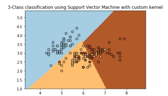
4. SVM分类

利用自定义核函数进行SVM分类，并将分类结果以及决策边界可视化展示出来。

import numpy as np
import matplotlib.pyplot as plt
from sklearn import svm, datasets

# import some data to play with
iris = datasets.load_iris()
X = iris.data[:, :2]  # we only take the first two features. We could
                      # avoid this ugly slicing by using a two-dim dataset
Y = iris.target


def my_kernel(X, Y):
    """
    We create a custom kernel:

                 (2  0)
    k(X, Y) = X  (    ) Y.T
                 (0  1)
    """
    M = np.array([[2, 0], [0, 1.0]])
    return np.dot(np.dot(X, M), Y.T)


h = .02  # step size in the mesh

# we create an instance of SVM and fit out data.
clf = svm.SVC(kernel=my_kernel)
clf.fit(X, Y)

# Plot the decision boundary. For that, we will assign a color to each
# point in the mesh [x_min, x_max]x[y_min, y_max].
x_min, x_max = X[:, 0].min() - 1, X[:, 0].max() + 1
y_min, y_max = X[:, 1].min() - 1, X[:, 1].max() + 1
xx, yy = np.meshgrid(np.arange(x_min, x_max, h), np.arange(y_min, y_max, h))
Z = clf.predict(np.c_[xx.ravel(), yy.ravel()])

# Put the result into a color plot
Z = Z.reshape(xx.shape)
plt.pcolormesh(xx, yy, Z, cmap=plt.cm.Paired)

# Plot also the training points
plt.scatter(X[:, 0], X[:, 1], c=Y, cmap=plt.cm.Paired, edgecolors='k')
plt.title('3-Class classification using Support Vector Machine with custom'
          ' kernel')
plt.axis('tight')
plt.show()

使用 datasets.load_iris() 加载了鸢尾花数据集。取数据集的前两个特征作为 X，标签作为 Y。

定义自定义核函数 my_kernel()：这个自定义核函数是一个线性组合的结果，将输入矩阵 X 与矩阵

Y 相乘，使用了一个特定的矩阵 M。

M 是一个二阶矩阵，[2,0],[0,1][2,0],[0,1]，用于定义自定义核的计算方式。

创建SVM分类器并使用自定义核函数进行训练：

使用 svm.SVC(kernel=my_kernel) 创建了一个支持向量机分类器，指定了自定义的核函数。

绘制决策边界：定义了 h 作为网格步长。创建了网格点 xx 和 yy，并利用 np.meshgrid() 创建了一

个二维网格。使用 clf.predict() 预测网格点的分类结果。将预测结果 Z 重塑成与网格相同的形状。

使用 plt.pcolormesh() 绘制了决策边界，用不同的颜色区分不同类别的预测结果。使用 plt.scatter()

绘制了训练数据点，用不同颜色表示不同类别，以及黑色边框表示支持向量。

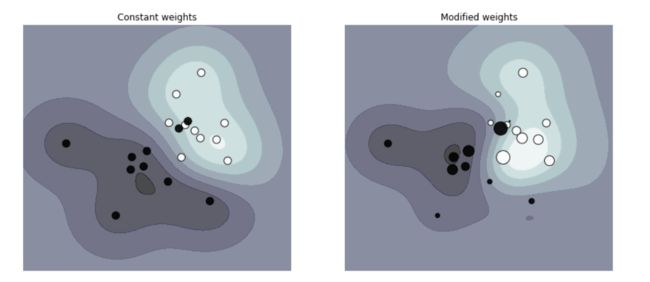
5. 权重的设置

比较在支持向量机分类器中考虑样本权重和不考虑样本权重时，对于异常样本（通过权重放大的样

本）对决策边界的影响。

import numpy as np
import matplotlib.pyplot as plt
from sklearn import svm


def plot_decision_function(classifier, sample_weight, axis, title):
    # plot the decision function
    xx, yy = np.meshgrid(np.linspace(-4, 5, 500), np.linspace(-4, 5, 500))

    Z = classifier.decision_function(np.c_[xx.ravel(), yy.ravel()])
    Z = Z.reshape(xx.shape)

    # plot the line, the points, and the nearest vectors to the plane
    axis.contourf(xx, yy, Z, alpha=0.75, cmap=plt.cm.bone)
    axis.scatter(X[:, 0], X[:, 1], c=y, s=100 * sample_weight, alpha=0.9,
                 cmap=plt.cm.bone, edgecolors='black')

    axis.axis('off')
    axis.set_title(title)


# we create 20 points
np.random.seed(0)
X = np.r_[np.random.randn(10, 2) + [1, 1], np.random.randn(10, 2)]
y = [1] * 10 + [-1] * 10
sample_weight_last_ten = abs(np.random.randn(len(X)))
sample_weight_constant = np.ones(len(X))
# and bigger weights to some outliers
sample_weight_last_ten[15:] *= 5
sample_weight_last_ten[9] *= 15

# for reference, first fit without class weights

# fit the model
clf_weights = svm.SVC()
clf_weights.fit(X, y, sample_weight=sample_weight_last_ten)

clf_no_weights = svm.SVC()
clf_no_weights.fit(X, y)

fig, axes = plt.subplots(1, 2, figsize=(14, 6))
plot_decision_function(clf_no_weights, sample_weight_constant, axes[0],
                       "Constant weights")
plot_decision_function(clf_weights, sample_weight_last_ten, axes[1],
                       "Modified weights")

plt.show()

生成数据和设置样本权重：创建了20个二维数据点，前10个点位于均值为1,11,1的正态分布中，后

10个点是从均值为0,00,0的正态分布中随机生成的。创建了对应的标签 y，前10个点标记为类别

1，后10个点标记为类别-1。创建了两种样本权重 sample_weight_last_ten 和

sample_weight_constant，sample_weight_last_ten 对后10个样本施加了较大的权重，尤其是第9

个样本的权重更大，而 sample_weight_constant 给所有样本赋予了相同的权重。

绘制决策边界：使用 svm.SVC() 创建了两个支持向量机分类器 clf_weights 和 clf_no_weights，分

别用于考虑权重和不考虑权重的情况。分别用 clf_weights.fit() 和 clf_no_weights.fit() 对数据进行拟

合，sample_weight 参数用于指定样本权重。

使用 plot_decision_function() 函数绘制了两个分类器的决策边界及数据点。其中，clf_weights 在

绘制中样本点的大小是基于其权重的，而 clf_no_weights 则是所有样本点大小均一。

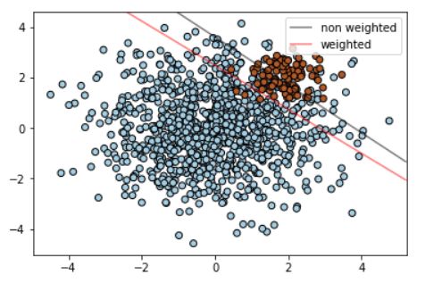
6. 类别不平衡

在面对类别不平衡的情况下，如何使用支持向量机（SVM）寻找最佳的分隔超平面，并且对比了

在样本类别权重不同的情况下得到的分隔超平面。

import numpy as np
import matplotlib.pyplot as plt
from sklearn import svm

# we create clusters with 1000 and 100 points
rng = np.random.RandomState(0)
n_samples_1 = 1000
n_samples_2 = 100
X = np.r_[1.5 * rng.randn(n_samples_1, 2),
          0.5 * rng.randn(n_samples_2, 2) + [2, 2]]
y = [0] * (n_samples_1) + [1] * (n_samples_2)

# fit the model and get the separating hyperplane
clf = svm.SVC(kernel='linear', C=1.0)
clf.fit(X, y)

# fit the model and get the separating hyperplane using weighted classes
wclf = svm.SVC(kernel='linear', class_weight={1: 10})
wclf.fit(X, y)

# plot separating hyperplanes and samples
plt.scatter(X[:, 0], X[:, 1], c=y, cmap=plt.cm.Paired, edgecolors='k')
plt.legend()

# plot the decision functions for both classifiers
ax = plt.gca()
xlim = ax.get_xlim()
ylim = ax.get_ylim()

# create grid to evaluate model
xx = np.linspace(xlim[0], xlim[1], 30)
yy = np.linspace(ylim[0], ylim[1], 30)
YY, XX = np.meshgrid(yy, xx)
xy = np.vstack([XX.ravel(), YY.ravel()]).T

# get the separating hyperplane
Z = clf.decision_function(xy).reshape(XX.shape)

# plot decision boundary and margins
a = ax.contour(XX, YY, Z, colors='k', levels=[0], alpha=0.5, linestyles=['-'])

# get the separating hyperplane for weighted classes
Z = wclf.decision_function(xy).reshape(XX.shape)

# plot decision boundary and margins for weighted classes
b = ax.contour(XX, YY, Z, colors='r', levels=[0], alpha=0.5, linestyles=['-'])

plt.legend([a.collections[0], b.collections[0]], ["non weighted", "weighted"],
           loc="upper right")
plt.show()

生成数据：创建了两个簇，一个包含1000个样本，另一个包含100个样本，两者分布不同。这些数

据点被标记为两个类别。

普通SVC和加权SVC：用 svm.SVC() 创建了一个支持向量机分类器 clf，它使用了普通的分类器参

数。使用带有权重参数 class_weight={1: 10} 的 svm.SVC() 创建了一个带权重的支持向量机分类

器 wclf。这个权重设置使得类别1（样本数少的类别）的误分类代价更高。

绘制数据和分隔超平面：使用 plt.scatter() 绘制了数据点，颜色代表了它们的真实类别。通过获取

当前轴对象 ax 的 x 和 y 轴的限制范围 xlim 和 ylim。创建了一个网格点坐标 xy，用于绘制决策边

界的等高线图。计算了普通SVC clf 和加权SVC wclf 的决策函数值，并绘制了它们对应的决策边

界，分别用黑色和红色表示。

7. 核函数

在不同情况下，不同类型的支持向量机核函数对非线性数据集的分类效果。三种核函数类型在决策

边界的表示和区域分隔上有所不同，其中多项式和径向基函数在处理非线性数据时通常效果更好。

# Code source: Gaël Varoquaux
# License: BSD 3 clause

import numpy as np
import matplotlib.pyplot as plt
from sklearn import svm


# Our dataset and targets
X = np.c_[(.4, -.7),
          (-1.5, -1),
          (-1.4, -.9),
          (-1.3, -1.2),
          (-1.1, -.2),
          (-1.2, -.4),
          (-.5, 1.2),
          (-1.5, 2.1),
          (1, 1),
          # --
          (1.3, .8),
          (1.2, .5),
          (.2, -2),
          (.5, -2.4),
          (.2, -2.3),
          (0, -2.7),
          (1.3, 2.1)].T
Y = [0] * 8 + [1] * 8

# figure number
fignum = 1

# fit the model
for kernel in ('linear', 'poly', 'rbf'):
    clf = svm.SVC(kernel=kernel, gamma=2)
    clf.fit(X, Y)

    # plot the line, the points, and the nearest vectors to the plane
    plt.figure(fignum, figsize=(4, 3))
    plt.clf()

    plt.scatter(clf.support_vectors_[:, 0], clf.support_vectors_[:, 1], s=80,
                facecolors='none', zorder=10, edgecolors='k')
    plt.scatter(X[:, 0], X[:, 1], c=Y, zorder=10, cmap=plt.cm.Paired,
                edgecolors='k')

    plt.axis('tight')
    x_min = -3
    x_max = 3
    y_min = -3
    y_max = 3

    XX, YY = np.mgrid[x_min:x_max:200j, y_min:y_max:200j]
    Z = clf.decision_function(np.c_[XX.ravel(), YY.ravel()])

    # Put the result into a color plot
    Z = Z.reshape(XX.shape)
    plt.figure(fignum, figsize=(4, 3))
    plt.pcolormesh(XX, YY, Z > 0, cmap=plt.cm.Paired)
    plt.contour(XX, YY, Z, colors=['k', 'k', 'k'], linestyles=['--', '-', '--'],
                levels=[-.5, 0, .5])

    plt.xlim(x_min, x_max)
    plt.ylim(y_min, y_max)

    plt.xticks(())
    plt.yticks(())
    fignum = fignum + 1
plt.show()

数据准备：创建了一个二维的数据集 X，包含16个点，每个点有两个特征。Y 是对应的标签，分为

两个类别。

使用不同核函数训练SVM模型：循环遍历三种核函数类型：线性、多项式和径向基函数

（RBF）。对于每个核函数类型，使用 svm.SVC() 创建了支持向量机分类器 clf。

绘制分类结果：对于每个核函数类型，创建了一个图像来展示数据点、支持向量以及决策边界。

使用 plt.scatter() 绘制了数据点和支持向量。使用 np.mgrid 生成网格点，用于绘制决策边界。

计算了决策函数的值 Z，并根据其值绘制了决策边界和区域的填充。

8. 单变量特征选择 

在支持向量分类器训练之前如何进行特征选择，以提高模型在数据上的分类性能。通过调整特征选

择的百分比，可以找到最佳的特征子集，以提高分类器的性能。

import numpy as np
import matplotlib.pyplot as plt
from sklearn import svm, datasets, feature_selection
from sklearn.model_selection import cross_val_score
from sklearn.pipeline import Pipeline

# Import some data to play with
digits = datasets.load_digits()
y = digits.target
# Throw away data, to be in the curse of dimension settings
y = y[:200]
X = digits.data[:200]
n_samples = len(y)
X = X.reshape((n_samples, -1))
# add 200 non-informative features
X = np.hstack((X, 2 * np.random.random((n_samples, 200))))

# Create a feature-selection transform and an instance of SVM that we
# combine together to have an full-blown estimator

transform = feature_selection.SelectPercentile(feature_selection.f_classif)

clf = Pipeline([('anova', transform), ('svc', svm.SVC(C=1.0))])

# Plot the cross-validation score as a function of percentile of features
score_means = list()
score_stds = list()
percentiles = (1, 3, 6, 10, 15, 20, 30, 40, 60, 80, 100)

for percentile in percentiles:
    clf.set_params(anova__percentile=percentile)
    # Compute cross-validation score using 1 CPU
    this_scores = cross_val_score(clf, X, y, n_jobs=1)
    score_means.append(this_scores.mean())
    score_stds.append(this_scores.std())

plt.errorbar(percentiles, score_means, np.array(score_stds))

plt.title(
    'Performance of the SVM-Anova varying the percentile of features selected')
plt.xlabel('Percentile')
plt.ylabel('Prediction rate')

plt.axis('tight')
plt.show()

准备数据：加载了手写数字数据集，并从中选择了前200个样本。设置了目标标签 y 和特征数据

X，并且在 X 中增加了200个非信息性特征以模拟高维数据。

创建管道：使用 feature_selection.SelectPercentile() 创建了一个特征选择转换器 transform，基于

单变量分析（ANOVA）的特征选择方法。创建了一个包含特征选择器和支持向量分类器管道 clf。

交叉验证评估特征选择的效果：设置不同的特征选择百分比（percentile），并使用交叉验证评估

每个百分比下分类器的性能。使用 cross_val_score() 计算了每个百分比下模型的交叉验证得分。

绘制结果：使用 plt.errorbar() 绘制了特征选择百分比与预测率的关系图。x轴是特征选择的百分

比，y轴是预测率，图中的误差条表示了交叉验证的标准差。

9. 参数C

参数C对支持向量机（SVM）分隔线的影响。C的值越大，模型越不信任数据的分布，只会考虑靠

近分隔线附近的点。C值越小，模型会考虑更多甚至全部的观测数据，从而影响分隔线的位置。

# Code source: Gaël Varoquaux
# Modified for documentation by Jaques Grobler
# License: BSD 3 clause

import numpy as np
import matplotlib.pyplot as plt
from sklearn import svm

# we create 40 separable points
np.random.seed(0)
X = np.r_[np.random.randn(20, 2) - [2, 2], np.random.randn(20, 2) + [2, 2]]
Y = [0] * 20 + [1] * 20

# figure number
fignum = 1

# fit the model
for name, penalty in (('unreg', 1), ('reg', 0.05)):

    clf = svm.SVC(kernel='linear', C=penalty)
    clf.fit(X, Y)

    # get the separating hyperplane
    w = clf.coef_[0]
    a = -w[0] / w[1]
    xx = np.linspace(-5, 5)
    yy = a * xx - (clf.intercept_[0]) / w[1]

    # plot the parallels to the separating hyperplane that pass through the
    # support vectors (margin away from hyperplane in direction
    # perpendicular to hyperplane). This is sqrt(1+a^2) away vertically in
    # 2-d.
    margin = 1 / np.sqrt(np.sum(clf.coef_ ** 2))
    yy_down = yy - np.sqrt(1 + a ** 2) * margin
    yy_up = yy + np.sqrt(1 + a ** 2) * margin

    # plot the line, the points, and the nearest vectors to the plane
    plt.figure(fignum, figsize=(4, 3))
    plt.clf()
    plt.plot(xx, yy, 'k-')
    plt.plot(xx, yy_down, 'k--')
    plt.plot(xx, yy_up, 'k--')

    plt.scatter(clf.support_vectors_[:, 0], clf.support_vectors_[:, 1], s=80,
                facecolors='none', zorder=10, edgecolors='k')
    plt.scatter(X[:, 0], X[:, 1], c=Y, zorder=10, cmap=plt.cm.Paired,
                edgecolors='k')

    plt.axis('tight')
    x_min = -4.8
    x_max = 4.2
    y_min = -6
    y_max = 6

    XX, YY = np.mgrid[x_min:x_max:200j, y_min:y_max:200j]
    Z = clf.predict(np.c_[XX.ravel(), YY.ravel()])

    # Put the result into a color plot
    Z = Z.reshape(XX.shape)
    plt.figure(fignum, figsize=(4, 3))
    plt.pcolormesh(XX, YY, Z, cmap=plt.cm.Paired)

    plt.xlim(x_min, x_max)
    plt.ylim(y_min, y_max)

    plt.xticks(())
    plt.yticks(())
    fignum = fignum + 1

plt.show()

这里有两种不同的C值进行展示：

unreg：对应C=1，表示较大的C值。reg：对应C=0.05，表示较小的C值。

对于每种C值：使用线性核（linear kernel）拟合了一个SVM模型。绘制了分隔超平面（separating

hyperplane）和间隔边界（margins）。使用不同的C值，调整了分隔超平面附近支持向量的数

量。图中的实线表示分隔超平面，虚线表示支持向量到分隔超平面的间隔边界。通过调整C值，可

以观察到分隔超平面对数据的敏感程度。较大的C值将更加强调分类边界附近的点，而较小的C值

则更加容忍，并考虑更多数据点。

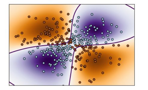
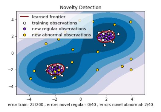
10. 非线性核（RBF）

图中展示了训练过程中学到的边界、训练数据、新的正常观测以及新的异常观测。这种模型可以用

于检测与训练数据集不同的新数据，并将其视为正常或异常观测。

import numpy as np
import matplotlib.pyplot as plt
import matplotlib.font_manager
from sklearn import svm

xx, yy = np.meshgrid(np.linspace(-5, 5, 500), np.linspace(-5, 5, 500))
# Generate train data
X = 0.3 * np.random.randn(100, 2)
X_train = np.r_[X + 2, X - 2]
# Generate some regular novel observations
X = 0.3 * np.random.randn(20, 2)
X_test = np.r_[X + 2, X - 2]
# Generate some abnormal novel observations
X_outliers = np.random.uniform(low=-4, high=4, size=(20, 2))

# fit the model
clf = svm.OneClassSVM(nu=0.1, kernel="rbf", gamma=0.1)
clf.fit(X_train)
y_pred_train = clf.predict(X_train)
y_pred_test = clf.predict(X_test)
y_pred_outliers = clf.predict(X_outliers)
n_error_train = y_pred_train[y_pred_train == -1].size
n_error_test = y_pred_test[y_pred_test == -1].size
n_error_outliers = y_pred_outliers[y_pred_outliers == 1].size

# plot the line, the points, and the nearest vectors to the plane
Z = clf.decision_function(np.c_[xx.ravel(), yy.ravel()])
Z = Z.reshape(xx.shape)

plt.title("Novelty Detection")
plt.contourf(xx, yy, Z, levels=np.linspace(Z.min(), 0, 7), cmap=plt.cm.PuBu)
a = plt.contour(xx, yy, Z, levels=[0], linewidths=2, colors='darkred')
plt.contourf(xx, yy, Z, levels=[0, Z.max()], colors='palevioletred')

s = 40
b1 = plt.scatter(X_train[:, 0], X_train[:, 1], c='white', s=s, edgecolors='k')
b2 = plt.scatter(X_test[:, 0], X_test[:, 1], c='blueviolet', s=s,
                 edgecolors='k')
c = plt.scatter(X_outliers[:, 0], X_outliers[:, 1], c='gold', s=s,
                edgecolors='k')
plt.axis('tight')
plt.xlim((-5, 5))
plt.ylim((-5, 5))
plt.legend([a.collections[0], b1, b2, c],
           ["learned frontier", "training observations",
            "new regular observations", "new abnormal observations"],
           loc="upper left",
           prop=matplotlib.font_manager.FontProperties(size=11))
plt.xlabel(
    "error train: %d/200 ; errors novel regular: %d/40 ; "
    "errors novel abnormal: %d/40"
    % (n_error_train, n_error_test, n_error_outliers))
plt.show()

准备数据：创建了两组数据：一组训练数据（X_train），一组用于检测的新数据（X_test）。

训练数据是由两组随机点构成，而新数据则包括了正常情况下的观测和异常情况下的观测。

训练模型：使用 svm.OneClassSVM() 创建了一个One-class SVM模型，使用RBF核，并进行了训

练。使用训练好的模型对训练数据、新的正常观测和新的异常观测进行了预测。

绘制结果：绘制了决策边界和间隔区域，显示了模型对正常和异常观测的区分。通过 plt.scatter()

绘制了训练数据、新的正常观测和新的异常观测。

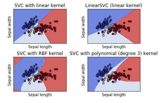
11. 不同类型的SVM

不同类型SVM模型在鸢尾花数据集上的分类效果。每个子图显示了模型在该数据集上学习到的决

策边界，有助于理解不同核函数和参数对分类边界的影响。

import numpy as np
import matplotlib.pyplot as plt
from sklearn import svm, datasets


def make_meshgrid(x, y, h=.02):
    """Create a mesh of points to plot in

    Parameters
    ----------
    x: data to base x-axis meshgrid on
    y: data to base y-axis meshgrid on
    h: stepsize for meshgrid, optional

    Returns
    -------
    xx, yy : ndarray
    """
    x_min, x_max = x.min() - 1, x.max() + 1
    y_min, y_max = y.min() - 1, y.max() + 1
    xx, yy = np.meshgrid(np.arange(x_min, x_max, h),
                         np.arange(y_min, y_max, h))
    return xx, yy


def plot_contours(ax, clf, xx, yy, **params):
    """Plot the decision boundaries for a classifier.

    Parameters
    ----------
    ax: matplotlib axes object
    clf: a classifier
    xx: meshgrid ndarray
    yy: meshgrid ndarray
    params: dictionary of params to pass to contourf, optional
    """
    Z = clf.predict(np.c_[xx.ravel(), yy.ravel()])
    Z = Z.reshape(xx.shape)
    out = ax.contourf(xx, yy, Z, **params)
    return out


# import some data to play with
iris = datasets.load_iris()
# Take the first two features. We could avoid this by using a two-dim dataset
X = iris.data[:, :2]
y = iris.target

# we create an instance of SVM and fit out data. We do not scale our
# data since we want to plot the support vectors
C = 1.0  # SVM regularization parameter
models = (svm.SVC(kernel='linear', C=C),
          svm.LinearSVC(C=C),
          svm.SVC(kernel='rbf', gamma=0.7, C=C),
          svm.SVC(kernel='poly', degree=3, C=C))
models = (clf.fit(X, y) for clf in models)

# title for the plots
titles = ('SVC with linear kernel',
          'LinearSVC (linear kernel)',
          'SVC with RBF kernel',
          'SVC with polynomial (degree 3) kernel')

# Set-up 2x2 grid for plotting.
fig, sub = plt.subplots(2, 2)
plt.subplots_adjust(wspace=0.4, hspace=0.4)

X0, X1 = X[:, 0], X[:, 1]
xx, yy = make_meshgrid(X0, X1)

for clf, title, ax in zip(models, titles, sub.flatten()):
    plot_contours(ax, clf, xx, yy,
                  cmap=plt.cm.coolwarm, alpha=0.8)
    ax.scatter(X0, X1, c=y, cmap=plt.cm.coolwarm, s=20, edgecolors='k')
    ax.set_xlim(xx.min(), xx.max())
    ax.set_ylim(yy.min(), yy.max())
    ax.set_xlabel('Sepal length')
    ax.set_ylabel('Sepal width')
    ax.set_xticks(())
    ax.set_yticks(())
    ax.set_title(title)

plt.show()

创建模型：创建了四种不同类型的SVM分类器：线性SVM、LinearSVC、RBF核SVM和三次多项

式核SVM。使用不同的核和参数对数据进行拟合。

12. 正则化参数 

通过不同的缩放方式（相对样本量或无缩放）展示了在不同训练集大小下，不同正则化参数C对模

型性能的影响。

# Author: Andreas Mueller 
#         Jaques Grobler 
# License: BSD 3 clause


import numpy as np
import matplotlib.pyplot as plt

from sklearn.svm import LinearSVC
from sklearn.model_selection import ShuffleSplit
from sklearn.model_selection import GridSearchCV
from sklearn.utils import check_random_state
from sklearn import datasets

rnd = check_random_state(1)

# set up dataset
n_samples = 100
n_features = 300

# l1 data (only 5 informative features)
X_1, y_1 = datasets.make_classification(n_samples=n_samples,
                                        n_features=n_features, n_informative=5,
                                        random_state=1)

# l2 data: non sparse, but less features
y_2 = np.sign(.5 - rnd.rand(n_samples))
X_2 = rnd.randn(n_samples, n_features // 5) + y_2[:, np.newaxis]
X_2 += 5 * rnd.randn(n_samples, n_features // 5)

clf_sets = [(LinearSVC(penalty='l1', loss='squared_hinge', dual=False,
                       tol=1e-3),
             np.logspace(-2.3, -1.3, 10), X_1, y_1),
            (LinearSVC(penalty='l2', loss='squared_hinge', dual=True,
                       tol=1e-4),
             np.logspace(-4.5, -2, 10), X_2, y_2)]

colors = ['navy', 'cyan', 'darkorange']
lw = 2

for fignum, (clf, cs, X, y) in enumerate(clf_sets):
    # set up the plot for each regressor
    plt.figure(fignum, figsize=(9, 10))

    for k, train_size in enumerate(np.linspace(0.3, 0.7, 3)[::-1]):
        param_grid = dict(C=cs)
        # To get nice curve, we need a large number of iterations to
        # reduce the variance
        grid = GridSearchCV(clf, refit=False, param_grid=param_grid,
                            cv=ShuffleSplit(train_size=train_size,
                                            n_splits=250, random_state=1))
        grid.fit(X, y)
        scores = grid.cv_results_['mean_test_score']

        scales = [(1, 'No scaling'),
                  ((n_samples * train_size), '1/n_samples'),
                  ]

        for subplotnum, (scaler, name) in enumerate(scales):
            plt.subplot(2, 1, subplotnum + 1)
            plt.xlabel('C')
            plt.ylabel('CV Score')
            grid_cs = cs * float(scaler)  # scale the C's
            plt.semilogx(grid_cs, scores, label="fraction %.2f" %
                         train_size, color=colors[k], lw=lw)
            plt.title('scaling=%s, penalty=%s, loss=%s' %
                      (name, clf.penalty, clf.loss))

    plt.legend(loc="best")
plt.show()

准备数据：生成了两个不同的数据集：一个稀疏（只有少数特征是有信息的）的l1数据集（X_1,

y_1）和一个非稀疏但特征较少的l2数据集（X_2, y_2）。

模型和参数设置：创建了两种不同的LinearSVC模型，一个使用L1正则化，另一个使用L2正则化。

对每个模型进行了参数网格搜索，调整正则化参数C的不同值。为了降低方差，使用了大量迭代次

数（n_splits=250）。

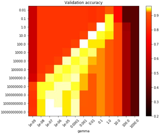
13. RBF核参数组合

通过网格搜索找到RBF核SVM模型的最佳参数组合，并通过可视化效果呈现不同参数对决策函数

的影响。

import numpy as np
import matplotlib.pyplot as plt
from matplotlib.colors import Normalize

from sklearn.svm import SVC
from sklearn.preprocessing import StandardScaler
from sklearn.datasets import load_iris
from sklearn.model_selection import StratifiedShuffleSplit
from sklearn.model_selection import GridSearchCV


# Utility function to move the midpoint of a colormap to be around
# the values of interest.

class MidpointNormalize(Normalize):

    def __init__(self, vmin=None, vmax=None, midpoint=None, clip=False):
        self.midpoint = midpoint
        Normalize.__init__(self, vmin, vmax, clip)

    def __call__(self, value, clip=None):
        x, y = [self.vmin, self.midpoint, self.vmax], [0, 0.5, 1]
        return np.ma.masked_array(np.interp(value, x, y))

# Load and prepare data set
#
# dataset for grid search

iris = load_iris()
X = iris.data
y = iris.target

# Dataset for decision function visualization: we only keep the first two
# features in X and sub-sample the dataset to keep only 2 classes and
# make it a binary classification problem.

X_2d = X[:, :2]
X_2d = X_2d[y > 0]
y_2d = y[y > 0]
y_2d -= 1

# It is usually a good idea to scale the data for SVM training.
# We are cheating a bit in this example in scaling all of the data,
# instead of fitting the transformation on the training set and
# just applying it on the test set.

scaler = StandardScaler()
X = scaler.fit_transform(X)
X_2d = scaler.fit_transform(X_2d)

# Train classifiers
#
# For an initial search, a logarithmic grid with basis
# 10 is often helpful. Using a basis of 2, a finer
# tuning can be achieved but at a much higher cost.

C_range = np.logspace(-2, 10, 13)
gamma_range = np.logspace(-9, 3, 13)
param_grid = dict(gamma=gamma_range, C=C_range)
cv = StratifiedShuffleSplit(n_splits=5, test_size=0.2, random_state=42)
grid = GridSearchCV(SVC(), param_grid=param_grid, cv=cv)
grid.fit(X, y)

print("The best parameters are %s with a score of %0.2f"
      % (grid.best_params_, grid.best_score_))

# Now we need to fit a classifier for all parameters in the 2d version
# (we use a smaller set of parameters here because it takes a while to train)

C_2d_range = [1e-2, 1, 1e2]
gamma_2d_range = [1e-1, 1, 1e1]
classifiers = []
for C in C_2d_range:
    for gamma in gamma_2d_range:
        clf = SVC(C=C, gamma=gamma)
        clf.fit(X_2d, y_2d)
        classifiers.append((C, gamma, clf))

# Visualization
#
# draw visualization of parameter effects

plt.figure(figsize=(8, 6))
xx, yy = np.meshgrid(np.linspace(-3, 3, 200), np.linspace(-3, 3, 200))
for (k, (C, gamma, clf)) in enumerate(classifiers):
    # evaluate decision function in a grid
    Z = clf.decision_function(np.c_[xx.ravel(), yy.ravel()])
    Z = Z.reshape(xx.shape)

    # visualize decision function for these parameters
    plt.subplot(len(C_2d_range), len(gamma_2d_range), k + 1)
    plt.title("gamma=10^%d, C=10^%d" % (np.log10(gamma), np.log10(C)),
              size='medium')

    # visualize parameter's effect on decision function
    plt.pcolormesh(xx, yy, -Z, cmap=plt.cm.RdBu)
    plt.scatter(X_2d[:, 0], X_2d[:, 1], c=y_2d, cmap=plt.cm.RdBu_r,
                edgecolors='k')
    plt.xticks(())
    plt.yticks(())
    plt.axis('tight')

scores = grid.cv_results_['mean_test_score'].reshape(len(C_range),
                                                     len(gamma_range))

# Draw heatmap of the validation accuracy as a function of gamma and C
#
# The score are encoded as colors with the hot colormap which varies from dark
# red to bright yellow. As the most interesting scores are all located in the
# 0.92 to 0.97 range we use a custom normalizer to set the mid-point to 0.92 so
# as to make it easier to visualize the small variations of score values in the
# interesting range while not brutally collapsing all the low score values to
# the same color.

plt.figure(figsize=(8, 6))
plt.subplots_adjust(left=.2, right=0.95, bottom=0.15, top=0.95)
plt.imshow(scores, interpolation='nearest', cmap=plt.cm.hot,
           norm=MidpointNormalize(vmin=0.2, midpoint=0.92))
plt.xlabel('gamma')
plt.ylabel('C')
plt.colorbar()
plt.xticks(np.arange(len(gamma_range)), gamma_range, rotation=45)
plt.yticks(np.arange(len(C_range)), C_range)
plt.title('Validation accuracy')
plt.show()

参数网格搜索：通过网格搜索调整了SVM模型中的C和gamma参数。参数范围选择了对数尺度下

的不同取值。使用了交叉验证进行参数选择，并记录了不同参数组合下的平均测试得分。

模型训练与可视化：对于全数据集和子数据集，分别训练了不同参数组合下的SVM模型。可视化

了不同参数组合下的决策函数效果，展示了每组参数在决策函数上的影响。

绘制图表：第一个图表绘制了决策函数的效果，展示了不同参数组合下的决策边界和数据点。第二

个图表是一个热力图，显示了不同参数组合下的交叉验证准确度。热力图中的颜色表示不同参数组

合下的验证准确度，让我们可以直观地观察参数对模型性能的影响。