SparkML(三)
分类
逻辑回归
在spark官方文档中,逻辑回归又分为二项式逻辑回归和多项式逻辑回归。
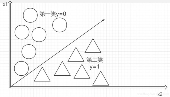
逻辑回归本质是线性回归,只是在特征到结果的过程上加上了一层映射。即首先需要把特征进行求和,然后将求和后的结果应用于一个g(z)函数,g(z)可以将值映射到0或者是1上面,这个函数就是Sigmoid函数,默认分类的值是0.5,超过0.5则类别为1,小于0.5类别为0。如下图
例子
import org.apache.spark.ml.classification.LogisticRegression

// Load training data
val training = spark.read.format("libsvm").load("data/mllib/sample_libsvm_data.txt")

val lr = new LogisticRegression()
  .setMaxIter(10)
  .setRegParam(0.3)
  .setElasticNetParam(0.8)

// Fit the model
val lrModel = lr.fit(training)

// Print the coefficients and intercept for logistic regression
println(s"Coefficients: ${lrModel.coefficients} Intercept: ${lrModel.intercept}")

// We can also use the multinomial family for binary classification
val mlr = new LogisticRegression()
  .setMaxIter(10)
  .setRegParam(0.3)
  .setElasticNetParam(0.8)
  .setFamily("multinomial")

val mlrModel = mlr.fit(training)

// Print the coefficients and intercepts for logistic regression with multinomial family
println(s"Multinomial coefficients: ${mlrModel.coefficientMatrix}")
println(s"Multinomial intercepts: ${mlrModel.interceptVector}")
在spark.ml逻辑回归中,可以通过使用二项式逻辑回归来预测二进制结果,或者在使用多项式逻辑回归时可以将其预测为多类结果。使用该family 参数在这两种算法之间进行选择,或者将其保留为未设置状态,Spark会推断出正确的变体。
决策树分类器
决策树(decision tree)是一种基本的分类与回归方法,这里主要介绍用于分类的决策树。决策树模式呈树形结构,其中每个内部节点表示一个属性上的测试,每个分支代表一个测试输出,每个叶节点代表一种类别。学习时利用训练数据,根据损失函数最小化的原则建立决策树模型;预测时,对新的数据,利用决策树模型进行分类。
使用该模型一般分为三个步骤:特征选择、决策树的生成和决策树的剪枝。
特征选择在于选取对训练数据具有分类能力的特征,这样可以提高决策树学习的效率。
从根结点开始,对结点计算所有可能的特征的信息增益,选择信息增益最大的特征作为结点的特征,由该特征的不同取值建立子结点,再对子结点递归地调用以上方法,构建决策树;直到所有特征的信息增均很小或没有特征可以选择为止,最后得到一个决策树。
决策树生成算法递归地产生决策树,直到不能继续下去为止。这样产生的树往往对训练数据的分类很准确,但对未知的测试数据的分类却没有那么准确,即出现过拟合现象。解决这个问题的办法是考虑决策树的复杂度,对已生成的决策树进行简化,这个过程称为剪枝。
例子
import org.apache.spark.ml.Pipeline
import org.apache.spark.ml.classification.DecisionTreeClassificationModel
import org.apache.spark.ml.classification.DecisionTreeClassifier
import org.apache.spark.ml.evaluation.MulticlassClassificationEvaluator
import org.apache.spark.ml.feature.{IndexToString, StringIndexer, VectorIndexer}

// Load the data stored in LIBSVM format as a DataFrame.
val data = spark.read.format("libsvm").load("data/mllib/sample_libsvm_data.txt")

// Index labels, adding metadata to the label column.
// Fit on whole dataset to include all labels in index.
val labelIndexer = new StringIndexer()
  .setInputCol("label")
  .setOutputCol("indexedLabel")
  .fit(data)
// Automatically identify categorical features, and index them.
val featureIndexer = new VectorIndexer()
  .setInputCol("features")
  .setOutputCol("indexedFeatures")
  .setMaxCategories(4) // features with > 4 distinct values are treated as continuous.
  .fit(data)

// Split the data into training and test sets (30% held out for testing).
val Array(trainingData, testData) = data.randomSplit(Array(0.7, 0.3))

// Train a DecisionTree model.
val dt = new DecisionTreeClassifier()
  .setLabelCol("indexedLabel")
  .setFeaturesCol("indexedFeatures")

// Convert indexed labels back to original labels.
val labelConverter = new IndexToString()
  .setInputCol("prediction")
  .setOutputCol("predictedLabel")
  .setLabels(labelIndexer.labelsArray(0))

// Chain indexers and tree in a Pipeline.
val pipeline = new Pipeline()
  .setStages(Array(labelIndexer, featureIndexer, dt, labelConverter))

// Train model. This also runs the indexers.
val model = pipeline.fit(trainingData)

// Make predictions.
val predictions = model.transform(testData)

// Select example rows to display.
predictions.select("predictedLabel", "label", "features").show(5)

// Select (prediction, true label) and compute test error.
val evaluator = new MulticlassClassificationEvaluator()
  .setLabelCol("indexedLabel")
  .setPredictionCol("prediction")
  .setMetricName("accuracy")
val accuracy = evaluator.evaluate(predictions)
println(s"Test Error = ${(1.0 - accuracy)}")

val treeModel = model.stages(2).asInstanceOf[DecisionTreeClassificationModel]
println(s"Learned classification tree model:\n ${treeModel.toDebugString}")
随机森林
随机森林 是决策树的集合体。随机森林结合了许多决策树,以减少过度拟合的风险。该spark.ml实现支持使用连续和分类功能对二进制和多类分类以及进行回归的随机森林。
随机森林是平均多个深决策树以降低方差的一种方法,其中,决策树是在一个数据集上的不同部分进行训练的。这是以偏差的小幅增加和一些可解释性的丧失为代价的,但是在最终的模型中通常会大大提高性能。
关键参数:
- numTrees(决策树的个数):增加决策树的个数会降低预测结果的方差,这样在测试时会有更高的accuracy。训练时间大致与numTrees呈线性增长关系。
- maxDepth:是指森林中每一棵决策树最大可能depth,在决策树中提到了这个参数。更深的一棵树意味模型预测更有力,但同时训练时间更长,也更倾向于过拟合。但是值得注意的是,随机森林算法和单一决策树算法对这个参数的要求是不一样的。随机森林由于是多个的决策树预测结果的投票或平均而降低而预测结果的方差,因此相对于单一决策树而言,不容易出现过拟合的情况。所以随机森林可以选择比决策树模型中更大的maxDepth。
例子
import org.apache.spark.ml.Pipeline
import org.apache.spark.ml.classification.{RandomForestClassificationModel, RandomForestClassifier}
import org.apache.spark.ml.evaluation.MulticlassClassificationEvaluator
import org.apache.spark.ml.feature.{IndexToString, StringIndexer, VectorIndexer}

// Load and parse the data file, converting it to a DataFrame.
val data = spark.read.format("libsvm").load("data/mllib/sample_libsvm_data.txt")

// Index labels, adding metadata to the label column.
// Fit on whole dataset to include all labels in index.
val labelIndexer = new StringIndexer()
  .setInputCol("label")
  .setOutputCol("indexedLabel")
  .fit(data)
// Automatically identify categorical features, and index them.
// Set maxCategories so features with > 4 distinct values are treated as continuous.
val featureIndexer = new VectorIndexer()
  .setInputCol("features")
  .setOutputCol("indexedFeatures")
  .setMaxCategories(4)
  .fit(data)

// Split the data into training and test sets (30% held out for testing).
val Array(trainingData, testData) = data.randomSplit(Array(0.7, 0.3))

// Train a RandomForest model.
val rf = new RandomForestClassifier()
  .setLabelCol("indexedLabel")
  .setFeaturesCol("indexedFeatures")
  .setNumTrees(10)

// Convert indexed labels back to original labels.
val labelConverter = new IndexToString()
  .setInputCol("prediction")
  .setOutputCol("predictedLabel")
  .setLabels(labelIndexer.labelsArray(0))

// Chain indexers and forest in a Pipeline.
val pipeline = new Pipeline()
  .setStages(Array(labelIndexer, featureIndexer, rf, labelConverter))

// Train model. This also runs the indexers.
val model = pipeline.fit(trainingData)

// Make predictions.
val predictions = model.transform(testData)

// Select example rows to display.
predictions.select("predictedLabel", "label", "features").show(5)

// Select (prediction, true label) and compute test error.
val evaluator = new MulticlassClassificationEvaluator()
  .setLabelCol("indexedLabel")
  .setPredictionCol("prediction")
  .setMetricName("accuracy")
val accuracy = evaluator.evaluate(predictions)
println(s"Test Error = ${(1.0 - accuracy)}")

val rfModel = model.stages(2).asInstanceOf[RandomForestClassificationModel]
println(s"Learned classification forest model:\n ${rfModel.toDebugString}")
梯度提升树分类器
梯度提升树(Gradient Boosting Decision Tree,GBDT)模型是一种基于提升方法的决策树改进的树模型,它训练多棵决策树,每一棵树学习的是之前的所有的树预测值与真实值之间的残差,最终将多棵树的打分进行叠加得出结果。GBDT控制树的规模保证每棵树只学习一部分的样本和特征,来防止过拟合,模型有较好的泛化性。
相比较GBDT算法只利用了一阶导数信息,XGBoost(Extreme Gradient Boosting)对损失函数做了二阶的泰勒展开,并在目标函数之外加入了正则项对整体求最优解,用以权衡目标函数的下降和模型的复杂程度,避免过拟合。
随机森林和GBDT都是基于决策树的集成模型,它们都可以简单直观地描述特征的非线性和特征之间的组合,有着不错的训练效果,同时可以较好地防止过拟合,两个模型的差别如下。
- GBDT每次只训练一个棵树,而随机森林可以同时并行训练多棵树,训练速度更快。
- 随机森林更不容易过拟合,随机森林中使用更多的树会降低过拟合风险,但是GBDT使用更多的树则会增加过拟合风险。
- 随机森林由于加入了随机抽样,相同样本和训练参数的多次训练结果会不同,训练过程不可复现,而GBDT每次的训练结果是相同的。
- 在MLlib实现中,随机森林可以处理二分类和多分类问题,而GBDT只能处理二分类问题。
- 随机森林和GBDT都是基于树模型的分类器,特征维度很大时,训练速度会非常慢,训练效果也较差,在实际的CTR预估中,一般会先将高维稀疏特征转化为低维稀疏特征,再用随机森林和GBDT进行训练。
例子
import org.apache.spark.ml.Pipeline
import org.apache.spark.ml.classification.{GBTClassificationModel, GBTClassifier}
import org.apache.spark.ml.evaluation.MulticlassClassificationEvaluator
import org.apache.spark.ml.feature.{IndexToString, StringIndexer, VectorIndexer}

// Load and parse the data file, converting it to a DataFrame.
val data = spark.read.format("libsvm").load("data/mllib/sample_libsvm_data.txt")

// Index labels, adding metadata to the label column.
// Fit on whole dataset to include all labels in index.
val labelIndexer = new StringIndexer()
  .setInputCol("label")
  .setOutputCol("indexedLabel")
  .fit(data)
// Automatically identify categorical features, and index them.
// Set maxCategories so features with > 4 distinct values are treated as continuous.
val featureIndexer = new VectorIndexer()
  .setInputCol("features")
  .setOutputCol("indexedFeatures")
  .setMaxCategories(4)
  .fit(data)

// Split the data into training and test sets (30% held out for testing).
val Array(trainingData, testData) = data.randomSplit(Array(0.7, 0.3))

// Train a GBT model.
val gbt = new GBTClassifier()
  .setLabelCol("indexedLabel")
  .setFeaturesCol("indexedFeatures")
  .setMaxIter(10)
  .setFeatureSubsetStrategy("auto")

// Convert indexed labels back to original labels.
val labelConverter = new IndexToString()
  .setInputCol("prediction")
  .setOutputCol("predictedLabel")
  .setLabels(labelIndexer.labelsArray(0))

// Chain indexers and GBT in a Pipeline.
val pipeline = new Pipeline()
  .setStages(Array(labelIndexer, featureIndexer, gbt, labelConverter))

// Train model. This also runs the indexers.
val model = pipeline.fit(trainingData)

// Make predictions.
val predictions = model.transform(testData)

// Select example rows to display.
predictions.select("predictedLabel", "label", "features").show(5)

// Select (prediction, true label) and compute test error.
val evaluator = new MulticlassClassificationEvaluator()
  .setLabelCol("indexedLabel")
  .setPredictionCol("prediction")
  .setMetricName("accuracy")
val accuracy = evaluator.evaluate(predictions)
println(s"Test Error = ${1.0 - accuracy}")

val gbtModel = model.stages(2).asInstanceOf[GBTClassificationModel]
println(s"Learned classification GBT model:\n ${gbtModel.toDebugString}")
线性支持向量机
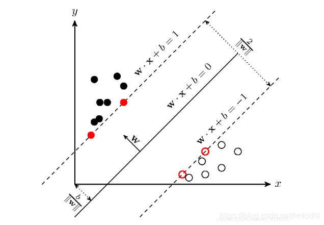
支持向量机,因其英文名为support vector machine,故一般简称SVM。SVM从线性可分情况下的最优分类面发展而来。最优分类面就是要求分类线不但能将两类正确分开(训练错误率为0),且使分类间隔最大。SVM考虑寻找一个满足分类要求的超平面,并且使训练集中的点距离分类面尽可能的远,也就是寻找一个分类面使它两侧的空白区域(margin)最大(即分类间隔最大化)。这两类样本中离分类面最近,且平行于最优分类面的超平面上的点,就叫做支持向量(下图中红色的点)。
超平面可以用分类函数表示 ,在进行分类的时候,遇到一个新的数据点x,将x代入f(x) 中,如果f(x)小于0则将x的类别赋为-1,如果f(x)大于0则将x的类别赋为1
例子
import org.apache.spark.ml.classification.LinearSVC

// Load training data
val training = spark.read.format("libsvm").load("data/mllib/sample_libsvm_data.txt")

val lsvc = new LinearSVC()
  .setMaxIter(10)
  .setRegParam(0.1)

// Fit the model
val lsvcModel = lsvc.fit(training)

// Print the coefficients and intercept for linear svc
println(s"Coefficients: ${lsvcModel.coefficients} Intercept: ${lsvcModel.intercept}")
相对于其余分类器
OneVsRest是机器学习简化的一个示例,它提供了可以有效执行二进制分类的基本分类器,从而执行了多分类。也称为“一对多”。
OneVsRest被实现为Estimator。对于基本分类器,它采用Classifierk个实例,并为k个类的每一个创建一个二进制分类问题。训练类别i的分类器以预测标签是否为i,从而将类别i与所有其他类别区分开。
预测是通过评估每个二进制分类器完成的,最可靠分类器的索引作为标签输出。
例子
import org.apache.spark.ml.classification.{LogisticRegression, OneVsRest}
import org.apache.spark.ml.evaluation.MulticlassClassificationEvaluator

// load data file.
val inputData = spark.read.format("libsvm")
  .load("data/mllib/sample_multiclass_classification_data.txt")

// generate the train/test split.
val Array(train, test) = inputData.randomSplit(Array(0.8, 0.2))

// instantiate the base classifier
val classifier = new LogisticRegression()
  .setMaxIter(10)
  .setTol(1E-6)
  .setFitIntercept(true)

// instantiate the One Vs Rest Classifier.
val ovr = new OneVsRest().setClassifier(classifier)

// train the multiclass model.
val ovrModel = ovr.fit(train)

// score the model on test data.
val predictions = ovrModel.transform(test)

// obtain evaluator.
val evaluator = new MulticlassClassificationEvaluator()
  .setMetricName("accuracy")

// compute the classification error on test data.
val accuracy = evaluator.evaluate(predictions)
println(s"Test Error = ${1 - accuracy}")
朴素贝叶斯
条件概率公式:
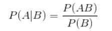
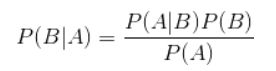
这个公式非常简单,就是计算在B发生的情况下,A发生的概率。但是很多时候,我们很容易知道P(A|B),需要计算的是P(B|A),这时就要用到贝叶斯定理:
举个简单的例子来说,下面这张表说明了各地区的人口构成:
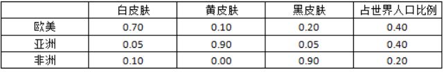
这个时候如果一个黑皮肤的人走过来(一个待分类项(0,0,1)),他是来自欧美,亚洲还是非洲呢?可以根据朴素贝叶斯分类进行计算:
欧美=0.30×0.90×0.20×0.40=0.0216
亚洲=0.95×0.10×0.05×0.40=0.0019
非洲=0.90×1.00×0.90×0.20=0.1620
即他来自非洲的可能性最大,来自欧美的可能性次之,来自亚洲的可能性最小,那么我们就判断他来自非洲,这和我们日常生活中的经验是一致的。
在spark中应用
import org.apache.spark.ml.classification.NaiveBayes
import org.apache.spark.ml.evaluation.MulticlassClassificationEvaluator

// Load the data stored in LIBSVM format as a DataFrame.
val data = spark.read.format("libsvm").load("data/mllib/sample_libsvm_data.txt")

// Split the data into training and test sets (30% held out for testing)
val Array(trainingData, testData) = data.randomSplit(Array(0.7, 0.3), seed = 1234L)

// Train a NaiveBayes model.
val model = new NaiveBayes()
  .fit(trainingData)

// Select example rows to display.
val predictions = model.transform(testData)
predictions.show()

// Select (prediction, true label) and compute test error
val evaluator = new MulticlassClassificationEvaluator()
  .setLabelCol("label")
  .setPredictionCol("prediction")
  .setMetricName("accuracy")
val accuracy = evaluator.evaluate(predictions)
println(s"Test set accuracy = $accuracy")