Batch Normalization、Layer Normalization、Group Normalization、Instance Normalization原理、适用场景和实际使用经验
Batch Normalization、Layer Normalization、Group Normalization、Instance Normalization原理、适用场景和使用经验
一、 简单介绍各种Normalization
先放一张来自Group Normalization原论文中的图,个人认为这个图很形象,以此图直观感受一下各种归一化的区别:
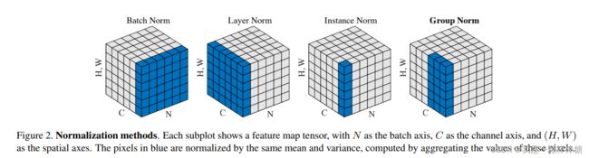
(注意:上图中,特征图的长和宽分别为W和H,由于我们的世界是3D的,直观只能展示3个维度,所以这里作者将H和W压缩成一个维度。则上图种每一个大方块展示的是一个Batch的特征图,其长宽高三个维度分别代表通道(Channel, C)、minibatch(BatchSize, N)、特征图(FeatureSize, (H,W)))
(1)Batch Normalization(上图左1):
- BN在Batch的方向上进行归一化,对于每一个channel的特征执行相同的操作,也就是说,这种归一化是通道间独立的
- 由于归一化操作会将参与归一化的特征映射到均值为0,方差为1的正态分布上。那么BN归一化之后,不同通道的特征的区分度减小(每个Channel都变成了 N ( 0 , 1 ) N~(0, 1) N (0,1)正态分布)。同时Batch内不同样本的特征仍然可区分
- 根据BN的特性我们很容易理解:由于各个样本间的特征区分度保留,而不同通道的特征区分度降低,这非常符合CV中的分类任务(一张图片里有一只猫,那么不同通道的特征都可以表达该信息,而Batch内另一张图片没有猫,这两个特征的区分度仍然很大)。
(2)Layer Normalization(上图左2):
- LN在Channel方向进行归一化,对于Batch内每一个样本执行相同操作,即样本间独立的
- 同样的,与BN相反,LN归一化之后,不同通道的特征的区分度不变。同时Batch内不同样本的特征区分度降低(每个样本都变成了 N ( 0 , 1 ) N~(0, 1) N (0,1)正态分布)
- 根据LN的特性我们很容易理解:由于不同通道的特征区分度保留,各个样本间的特征区分度消失,这非常符合NLP中的语义特征(相同的字在不同的上下文中,有不同的含义,但是每个句子之间不需要有明显的差别)。
(3)Instance Normalization(上图左3):
- IN在每个样本的每个Channel内部进行归一化,即样本和通道同时独立的
- 同样的,IN归一化之后,不同像素的特征的区分度不变。同时Batch内不同样本以及同一样本的不同通道的特征区分度都降低(每个样本和通道都变成了 N ( 0 , 1 ) N~(0, 1) N (0,1)正态分布)
- IN一般用于生成任务和风格迁移任务,因为这种任务会对细节特征有高要求,直观可以理解为更细粒度的特征区分要求
(4)Group Normalization(上图左4):
- GN在Channel方向分组(group),然后在每个group内进行归一化
- 有了前面的介绍,其实GN直观上像是LN的和IN的折中,当分组数量为1时,GN就变成了LN,分组数量等于通道数时,GN就变成了IN。
二、各种归一化的详细介绍
1. Batch Normalization
(1)论文出处:链接
(2)原理
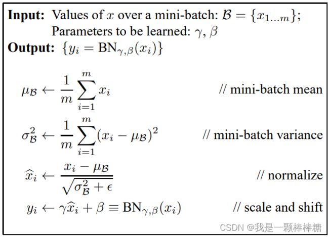
核心过程即如下算法流程:
- 对于输入的所有 x i x_i xi,计算集合 B = { x 1 , x 2 , x 3 , ⋯ , x i } B = \{ x_1,x_2,x_3,\cdots,x_i\} B={x1,x2,x3,⋯,xi}的均值 μ B \mu_B μB和方差 σ B 2 \sigma_B^2 σB2
- 进行归一化操作
- 值得一提的是,BN中最后还有一个线性仿射变换,即有一个缩放参数 γ \gamma γ和平移参数 β \beta β,这两个参数是可学习的。这是因为不同的batch的分布可能是不一样的,纵使BN可以将同一个Batch的分布拉到同一分布,但是不能保证对所有batch的数据都合适
(3)使用场景
BN可以加快深度神经网络的训练速度(可以在训练时使用更高的学习率,因为数据归一化之后,不会使得梯度有太大的波动),并给网络的权重提供了正则化,可以一定程度上防止过拟合
BN可以在任何场景下使用,你可以把它当作一个默认操作,后面再调整,但是这里要说一下调整的依据:
- BN不适用于Batchsize很小的情况,这里再放一张GN论文中的图:
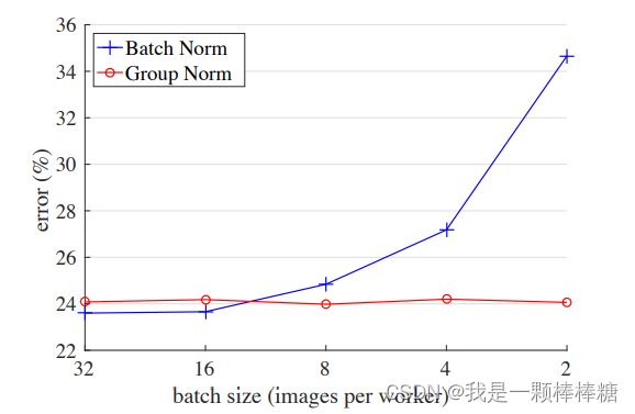
随着Batchsize减小,BN的性能越来越差,直观理解起来其实很简单:就是因为小的Batch中的数据并不能很好的表达一个分布,这就导致了梯度波动变大了,所以BN带来的正则防止过拟合性能就会降低。
(4)Pytorch 使用方法
>>> # With Learnable Parameters
>>> m = nn.BatchNorm2d(100)
>>> # Without Learnable Parameters
>>> m = nn.BatchNorm2d(100, affine=False)
>>> input = torch.randn(20, 100, 35, 45)
>>> output = m(input)
前文已经大致描述了其他各种归一化方法的操作,后文就不再赘述了
2. Layer Normalization
(1)论文出处:链接
(2)使用场景
- LN大部分用于NLP任务,可以作为该类任务的默认选项
- 当任务本身不需要太多词级语义信息,可以考虑使用BN
- LN可以用于小Batchsize下的CV任务(风格迁移、图像生成),可以提升效果
(3)Pytorch 使用方法
>>> # NLP Example
>>> batch, sentence_length, embedding_dim = 20, 5, 10
>>> embedding = torch.randn(batch, sentence_length, embedding_dim)
>>> layer_norm = nn.LayerNorm(embedding_dim)
>>> # Activate module
>>> layer_norm(embedding)
>>>
>>> # Image Example
>>> N, C, H, W = 20, 5, 10, 10
>>> input = torch.randn(N, C, H, W)
>>> # Normalize over the last three dimensions (i.e. the channel and spatial dimensions)
>>> # as shown in the image below
>>> layer_norm = nn.LayerNorm([C, H, W])
>>> output = layer_norm(input)
3. Instance Normalization
(1)论文出处:链接
(2)使用场景
- IN大部分用于图像生成和风格迁移任务,可以作为该类任务的默认选项
(3)Pytorch 使用方法
>>> # Without Learnable Parameters
>>> m = nn.InstanceNorm2d(100)
>>> # With Learnable Parameters
>>> m = nn.InstanceNorm2d(100, affine=True)
>>> input = torch.randn(20, 100, 35, 45)
>>> output = m(input)
4. Group Normalization
(1)论文出处:链接
(2)使用场景
- GN作为在小Batchsize下的调整选项,可以提升模型性能(亲测有效)
(3)Pytorch 使用方法
>>> input = torch.randn(20, 6, 10, 10)
>>> # Separate 6 channels into 3 groups
>>> m = nn.GroupNorm(3, 6)
>>> # Separate 6 channels into 6 groups (equivalent with InstanceNorm)
>>> m = nn.GroupNorm(6, 6)
>>> # Put all 6 channels into a single group (equivalent with LayerNorm)
>>> m = nn.GroupNorm(1, 6)
>>> # Activating the module
>>> output = m(input)