手把手神经网络讲解和无调包实现系列（2）Softmax回归【R语言】【小白学习笔记】

在第一期我们讲解并实现了最基本的线性回归，这一期我们会紧接着从回归问题讲到分类问题，而这时我们需要在线性回归模型的基础上增添一些元素，也就是 激活函数【activation function】从而让我们的模型可以解决非线性的数据和分类的问题。

往期精彩：
手把手神经网络讲解和无调包实现系列（1）线性回归【R语言】【小白学习笔记】

一· 模型讲解

1 假设函数 【Hypothesis Function】

假设一组数据里面有n个数据点和4个特征和3个分类变量【categorical variable】目标。我们的目的是要通过建立一个数学模型来学习现有数据的特征并最终能准确的预测目标变量。由于分类变量跟连续变量不同和特殊性，我们需要在训练模型前对分类变量进行one-hot编码【one-hot encoding】。让我们举个简单的例子，比如我们的目标分类变量是去分辨水果【苹果，香蕉，橙子】，那one-hot编码后的变量会变成这样
【：（1，0，0）， ：（0，1，0），：（0，0，1）】。
完成以上编码后，接下来会开始讲解Softmax回归模型的理论。按照神经网络的框架来的话， Softmax回归其实就是个只有一层的全链接层（稠密层）【fully connected/dense layer】的神经网络。
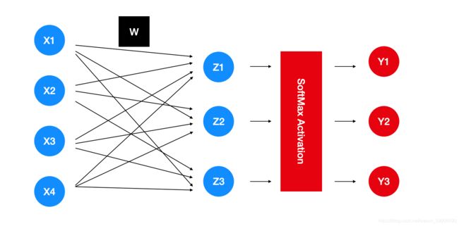上面提到的数据案例直接带入模型就会像图表展示那样，其中图表没有把偏差画出来，但是我们默认偏差的存在，红色所代表的步骤会在激活函数小节中说明。
把图表中的蓝色步骤写成数学公式的话，
$$\begin{gathered} z_1=x_1{w}_{11}+x_2{w}_{12}+x_3{w}_{13}+x_4{w}_{14}+b_1, \\ {z}_2=x_1{w}_{21}+x_2{w}_{22}+x_3{w}_{23}+x_4{w}_{24}+b_2, \\ {z}_3=x_1{w}_{31}+x_2{w}_{32}+x_3{w}_{33}+x_4{w}_{34}+b_3, \end{gathered}$$
其中$w$是模型的权重参数【weights】，$b$是偏差【bias/intercept】。

为了让计算更简洁，把公式矢量化，
$$Z=XW+b,$$
这里$Z$就是我们的假设函数。

同时也会把偏差值藏进$w$里面进一步的简化，
$$\boxed{Z=XW},$$
如果按上面的数据案例的话，
$Z=\left[\begin{array}{ccc}1& 0& 0\\ 0& 1& 0\\ ...& ...& ...\\ 0& 0& 1\end{array}\right],X=\left[\begin{array}{ccccc}1& x_{11}& x_{12}& x_{13}& x_{14}\\ ...& ...& ...& ...& ...\\ 1& x_{n1}& x_{n2}& x_{n3}& x_{n4}\end{array}\right],W=\left[\begin{array}{ccc}{b}_1& b_2& b_3\\ w_{11}& w_{21}& w_{31}\\ w_{12}& w_{22}& w_{32}\\ w_{13}& w_{23}& w_{33}\\ w_{14}& w_{24}& w_{34}\end{array}\right]$。
广泛化的话，假如我们的数据拥有n个数据点，m个特征，K个分类变量，那$X$会是一个$n\ast （m+1）$的矩阵，$W$会是一个$（m+1）\ast K$的矩阵，最后$Z$会是一个$n\ast K$的矩阵。

2 激活函数【Activation Function】

如果我们使用的是线性回归的话，上面的假设函数就已经足够了。但是我们这次要解决的是分类问题，因此我们需要一些额外的步骤去转变线性公式从而计算出新的量化值来预测分类变量，而概率就自然而然地变成最合适的量化值！因此第一步算出$Z$后，下一步会需要一个新的函数去转变成概率，而这个步骤通常叫作激活（就是上图中的红色部分），而这次用到的激活函数是Softmax函数，最早在1959年一名叫R. Duncan Luce的社会科学家所使用，我们模型的名称也就是从这而来的。函数公式如下，

$$\boxed{{\hat{y}}_j=\frac{exp(Z_j)}{{\sum }_{j=1}^{K}exp(Z_j)}},$$
其中 ${\hat{y}}_j$是计算出的预测概率, $K$代表目标分类变量的数量, $j$是目标分类变量的索引。分母是确保转换的概率只能有0-1的范围。

3 损失函数【Loss Function】

在训练模型时，我们会需要损失函数来量化预测的误差，同时分类问题所用到的损失函数和回归问题的也会有所不同。当计算出以下真实分类的概率时，
$$P(\hat{Y}|X)=\prod _{i=1}^{n}P({\hat{y}}^{(i)}|x^{(i)}).$$

根据极大似然估计【maximum likelihood estimation】的逻辑，我们的目标是把$P(\hat{Y}|X)$ 最大化，但是由于$P(\hat{Y}|X)$ 是一系列乘积所组成，求导会变得异常困难，这时通过$log$(这里$log$ 指的是自然对数$ln$ ） 特性，我们可以把乘积转化成总和,同时因为$log$ 是一个单调上升函数【monotonic increasing function】，因此通过对数似然值【log-likelihood】所得到的答案会同时解答原本的似然值。最后由于机器学习的习惯是按最小化问题的视角，当我们要最大化$P(\hat{Y}|X)$ 时，相对地就是把$-logP(\hat{Y}|X)$最小化，

$$-logP(\hat{Y}|X)=\sum _{i=1}^n-logP({\hat{y}}^{(i)}|x^{(i)})=\sum _{i=1}^{n}l({\hat{y}}^{(i)},y^{(i)}),$$
这里我们终于确定了我们的损失函数$l({\hat{y}}^{(i)},y^{(i)})$，
$$\boxed{l({\hat{y}}^{(i)},y^{(i)})=-\sum _{j=1}^K{y}_{j}log{\hat{y}}_j}。$$
有几点特别值得注意，第一上面的损失函数就是Shannon信息论里面著名的交叉熵【cross entropy】。第二点是$y_j$是我们的真实分类目标，在最开始时我们对分类变量使用了one-hot编码（如【：（1，0，0）， ：（0，1，0），：（0，0，1）】），因此当计算$y_{j}log{\hat{y}}_j$时，只有正确的分类预测概率才会得以保存，其它非正确的分类就会等于$0$。

4 随机梯度下降法推导 【Stochastic Gradient Decent】

这次我们同样会使用小批随机梯度下降法找出最优解的模型参数$W$，因此需要解出偏导$\frac{\partial l}{\partial W}$。不过要注意的是损失函数$l$是一个复合函数，要从$\hat{y}$到$Z$再到$W$这样一步一步往下套，写成数学等式的话就是$l({\hat{y}}^{(i)},y^{(i)})=l(\text{SoftMax}(Z(W)),y^{(i)})$，这时链式法则【chain rule】就变得非常方便，
$$\frac{\partial l}{\partial W}=\frac{\partial l}{\partial Z}\frac{\partial Z}{\partial W}.$$
在求导前，先把损失函数转化成$Z$的函数，
$$\begin{gathered} l({\hat{y}}^{(i)},y^{(i)})=-\sum _{j=1}^K{y}_{j}log\frac{exp(Z_j)}{{\sum }_{k=1}^{K}exp(Z_k)}, \\ l({\hat{y}}^{(i)},y^{(i)})=-\sum _{j=1}^K{y}_j{Z}_j+\sum _{j=1}^K{y}_{j}log(\sum _{k=1}^{K}exp(Z_k)), \end{gathered}$$
在第二步中，我们再次使用了log的特性来简化公式，然后这里有两个索引$j$和$k$，它们都是在求分类变量的总和只不过需要区分开来才使用不同的索引。更重要的是${\sum }_{j=1}^K{y}_j$等于1（原因是one-hot编码），$l$的最终公式如下，
$$l=log(\sum _{k=1}^{K}exp(Z_k))-\sum _{j=1}^K{y}_j{Z}_j.$$
剩下的便是求导，
$$\begin{gathered} \frac{\partial l}{\partial Z}=\frac{1}{{\sum }_{k=1}^{K}exp(Z_k)}exp(Z_k)-y_j=\text{Softmax}(Z_j)-y_j={\hat{y}}_j-y_j， \\ \frac{\partial Z}{\partial W}=\frac{\partial }{\partial W}(X^{(i)}W)=X^{(i)}， \\ \boxed{\frac{\partial l}{\partial W}=\frac{\partial l}{\partial Z}\frac{\partial Z}{\partial W}=X^{(i)}({\hat{y}}_j-y_j)}. \end{gathered}$$
眼利的同学会发现得出的偏导不就是跟线性回归模型时的一模一样吗！是的，所有指数族分布【exponential family distribution】模型的偏导都会是这个结果，唯一的变化在$\hat{y}$。

接下来按照随机梯度下降法来更新模型的参数 $W$，
$$\begin{gathered} W=W-\frac{\eta }{\beta }\sum _{i\in \beta }{\nabla }_W{l}^{(i)}(W)， \\ \boxed{W=W-\frac{\eta }{\beta }\sum _{i\in \beta }{X}^{(i)}({\hat{y}}_j-y_j)}, \end{gathered}$$
这里$\eta$是学习率【learning rate】，$\beta$ 是批量【batch size】。

5 算法总结

把所需要实现的步骤重新总结如下，

1. 随机生成权重参数$(W,b)$。
2. 计算假设函数$Z=XW$。
3. 激活$Z$也就是算出$\hat{y}=\frac{exp(Z_j)}{{\sum }_{j=1}^{K}exp(Z_j)}$.
4. 运算一步小批随机梯度下降法.
5. 更新$(W,b)$, $W=W-\frac{\eta }{\beta }{\sum }_{i\in \beta }{X}^{(i)}({\hat{y}}_j-y_j)$
6. 重复2-5直到达到预设的周期或者其它预设情形。

二· 数据

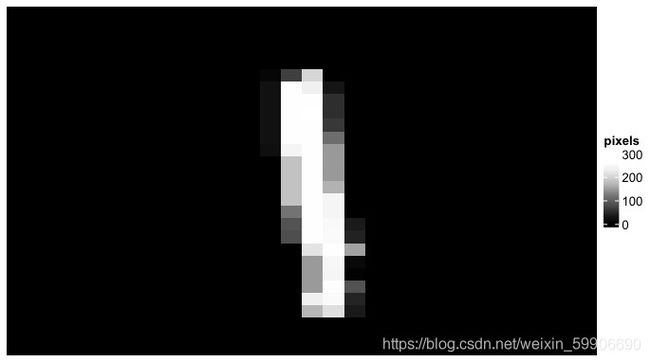
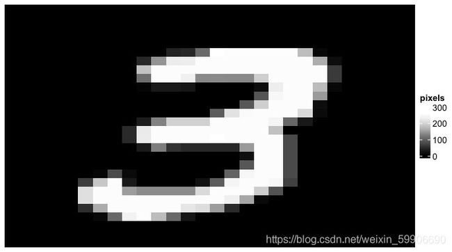
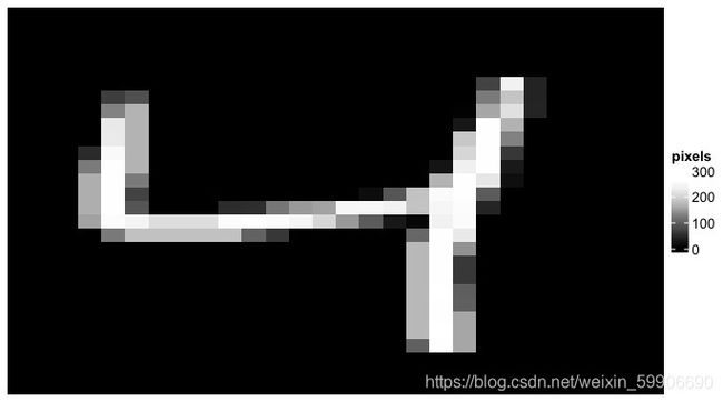
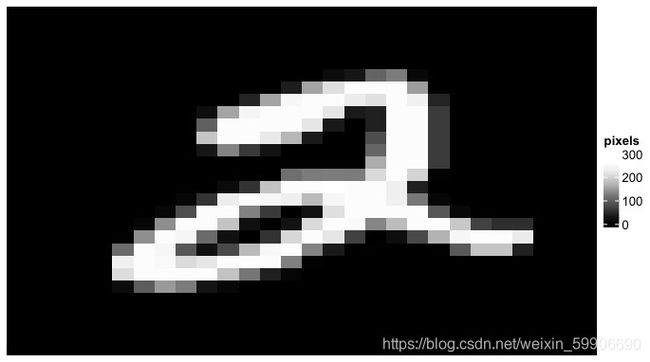
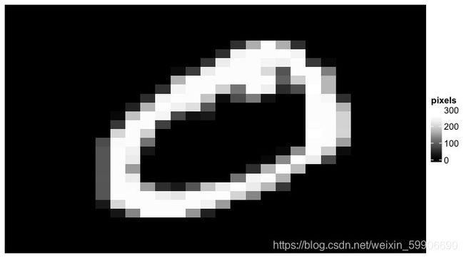
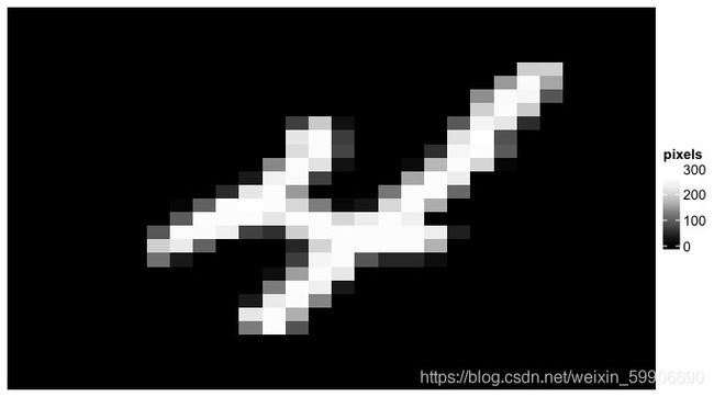
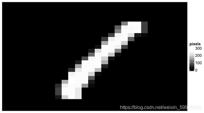
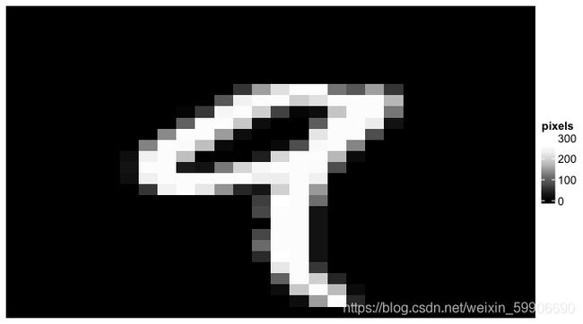
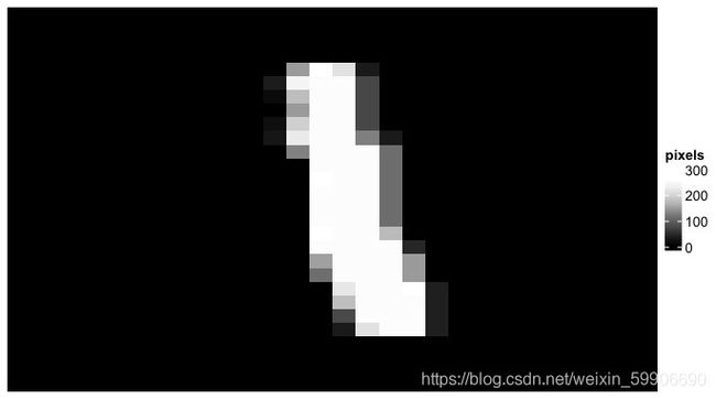
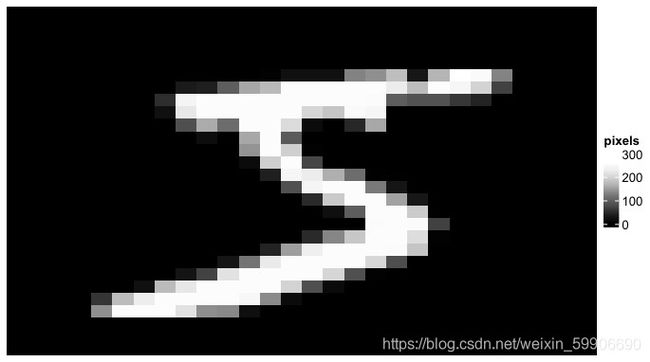
讲解完模型原理后，我们会首先了解本次所使用的数据，这次是著名的手写数字（0-9）分类MNIST数据库。每一个数据点是一张28x28的黑白图片，我们的目标是利用Softmax回归来实现简单的计算机视觉【computer vision】模型，也就是让AI来分别图片所写的是0到9中的哪一个数字。第一步将会是从Keras包中下载MNIST数据库和数据的可视化。

library(tidyverse)
library(matrixStats)
library(tensorflow)
library(keras)

library(RColorBrewer)
# install.packages('ComplexHeatmap')
library(ComplexHeatmap)


# ---------------------------- Load the Data -------------------------------
# Digit dataset
mnist = dataset_mnist()
X_train = mnist$train$x
Y_train = mnist$train$y
X_test = mnist$test$x
Y_test = mnist$test$y

# VIZ the image:
PlotImage = function(image_array) {
  digit_color = colorRampPalette(rev(brewer.pal(n=9, 
                                                name = "Greys")))(100)
  Heatmap(image_array, name= 'pixels',
          col = digit_color,
          cluster_rows = F, cluster_columns = F,
          border = F, column_names_rot = 90
  )
}

for (i in 1:10) {
  image = X_train[i, , ]
  print(PlotImage(image))  
}

–代码输出：










在用原数据训练模型之前，原数据还需要更进一步的处理。第一步是把所有28x28的图片数据压平【flatten】成nxm的矩阵，其中n代表图片数量而m代表$28\ast 28=784$个像素特征。压平数据后，下一步是让数据除以最高像素值（255）来标准化成0-1的范围。剩下要注意的是通过在压平的矩阵的第一列前添加全是1 的列向量从而让偏差值$b$融入$W$里面。最后是对图片的数字目标进行one-hot编码（使用的是Keras里面的’to_categorical’函数）。

# ---------------------------- Data Processing -------------------------------
## Flatten the 2D image into 1D features:
X_train_mat = matrix(0,  nrow = nrow(X_train), ncol = 28*28 )
for (i in 1:nrow(X_train)){
  # also normalize the pixel value by dividing 255
  X_train_mat[i, ] = matrix(X_train[i, , ], ncol = 28*28, byrow = TRUE) / 255
}

X_test_mat = matrix(0, nrow = nrow(X_test), ncol = 28*28 )
for (i in 1:nrow(X_test)){
  # also normalize the pixel value by dividing 255
  X_test_mat[i, ] = matrix(X_test[i, , ], ncol = 28*28, byrow = TRUE) / 255
}

## Add dummy col of value 1 to X for embedding the bias term:
X_train_mat = cbind(rep(1, nrow(X_train_mat)), X_train_mat)
X_test_mat = cbind(rep(1, nrow(X_test_mat)), X_test_mat)

## One-hot encoding for the Label:
Y_train_oh = to_categorical(Y_train)
Y_test_oh = to_categorical(Y_test)

# check training data dimension
dim(X_train_mat)
dim(Y_train_oh)

三· 模型实现

在完成数据的转化后，就让我们开始实现Softmax回归模型。先从简单的假设函数和Softmax激活函数开始。

Hypothesis = function(X, w) {
  ## Hypothesis function: Z = XW + b
  # Notice: b is already embedded within W as the first column
  return(X %*% w )
}

Softmax = function(Z){
  ## Softmax activation: exp(Z) / Row Summation (exp(Z)) 
  return( exp(Z) / rowSums(exp(Z)) )
}

接下来把损失函数交叉熵也写出来。同时我们会增添一个可以计算出预测准确率的助理函数。注意的是交叉熵所需的是one-hot编码后的目标值$Y_{oh}$而预测准确率的函数所需的是one-hot编码前的原目标值$Y$！

CrossEntropy = function(Y_hat, Y_oh){
  ## Loss function: l(yhat, y) = -summation(yj log yhatj)
  # NOTEL Groud Truth Y need to be one-hot encoded.
  # using the Ground Truth target as index to only select the nonzero class
  # [using normal element wise multiplication instead of matrix multiplication]
  return(-rowSums(log(Y_hat) * Y_oh))
}

ComputeAccuracy = function(Y_hat, Y){
  ## Compute the Accuracy
  # need to subtract 1 here because the target starts with 0!
  pred = apply(Y_hat, MARGIN = 1, FUN = function(x) which.max(x) - 1)
  acc = sum(pred == Y) / length(Y)
  return(acc)
}

剩下的是写出随机梯度下降法的R函数。像往常一样，在运行矩阵乘法时，一定要注意相乘矩阵的尺寸，要不然会直接出bug。比如$X_{batch}$是一个$\beta \ast (m+1)$的矩阵和${\hat{Y}}_{batch}-Y_{batch}$ 的结果是一个$\beta \ast K$的矩阵，最终目标是要更新$W$而$W$是一个$(m+1)\ast K$的矩阵。因此其中的一个方法是转置$X_{batch}$成$(m+1)\ast \beta$的矩阵，这样就能和${\hat{Y}}_{batch}-Y_{batch}$ 的结果无误的相乘。

SGD = function(X, Y_oh, w, lr, batch_size){
  ## minibatch stochastic gradient descent
  
  # Minibatch sampling:
  batch_ind = sample(nrow(X), batch_size, replace = FALSE)
  X_batch = X[batch_ind, ]
  Y_batch = Y_oh[batch_ind, ]
    
  # Compute gradient for the batch sample:
  Z_batch = Hypothesis(X_batch, w)
  Y_hat_batch = Softmax(Z_batch)
  # transpose X for correct dimension
  w_grad = t(X_batch) %*% (Y_hat_batch - Y_batch) 
  
  # Update w
  w = w - lr/batch_size * w_grad
  
  return(w)

}

码好所有需要的函数后，我们就可以随机生成模型所需的参数，然后开始训练模型。

# ------------------------- Initiate Models Parameters ---------------------------
n = nrow(X_train_mat) # num of training data points
m = ncol(X_train_mat) # num of features
k = ncol(Y_train_oh) # num of target classes

# Dim(w) = num of features * num of Target Classes
# note: b is also embedded within W as the first column
w = matrix(rnorm(m*k, mean = 0, sd = 0.01), 
           nrow = m, ncol = k, byrow = TRUE )
#
batch_size = 512
lr = 0.5
num_epoch = 50
#
net = Hypothesis
active = Softmax 
loss = CrossEntropy
#
w_list = list()
l_list = list()
acc_list = list()

# ------------------------------ Train the models --------------------------------
for (epoch in 1:num_epoch ){
  # Update parameters w:
  w = SGD(X_train_mat, Y_train_oh, w, lr, batch_size)
  Y_hat = active(net(X_train_mat, w))
  l = loss(Y_hat, Y_train_oh)
  acc_train = ComputeAccuracy(Y_hat, Y_train)
  
  # Compute test data accuracy:
  Y_hat_test = active(net(X_test_mat, w))
  acc_test = ComputeAccuracy(Y_hat_test, Y_test)
  ## Accumulate parameters, loss, and accuracy:
  w_list[[epoch]] = w
  l_list[[epoch]] = l
  acc_list[[epoch]] = acc_test
  
  print(str_c('epoch ', epoch, ' Loss: ', mean(l), 
              ' Train Accuracy: ', acc_train, ' Test Accuracy: ', acc_test ))
  
}

–代码输出：

[1] "epoch 1 Loss: 2.01185957862662 Train Accuracy: 0.3933 Test Accuracy: 0.3932"
[1] "epoch 2 Loss: 1.79866336994313 Train Accuracy: 0.5837 Test Accuracy: 0.5815"
[1] "epoch 3 Loss: 1.60035098466163 Train Accuracy: 0.692483333333333 Test Accuracy: 0.6981"
[1] "epoch 4 Loss: 1.45199775782509 Train Accuracy: 0.753166666666667 Test Accuracy: 0.7591"
[1] "epoch 5 Loss: 1.32667656580226 Train Accuracy: 0.805016666666667 Test Accuracy: 0.81"
[1] "epoch 6 Loss: 1.23351659868024 Train Accuracy: 0.77195 Test Accuracy: 0.7797"
[1] "epoch 7 Loss: 1.15247059426567 Train Accuracy: 0.790816666666667 Test Accuracy: 0.7965"
[1] "epoch 8 Loss: 1.08940996066825 Train Accuracy: 0.822066666666667 Test Accuracy: 0.832"
[1] "epoch 9 Loss: 1.03435513731771 Train Accuracy: 0.79235 Test Accuracy: 0.7997"
[1] "epoch 10 Loss: 0.992790215169106 Train Accuracy: 0.795583333333333 Test Accuracy: 0.8038"
[1] "epoch 11 Loss: 0.946572561174173 Train Accuracy: 0.824333333333333 Test Accuracy: 0.8357"
[1] "epoch 12 Loss: 0.909750711598293 Train Accuracy: 0.824633333333333 Test Accuracy: 0.831"
[1] "epoch 13 Loss: 0.87881802974624 Train Accuracy: 0.821616666666667 Test Accuracy: 0.8289"
[1] "epoch 14 Loss: 0.856014529247105 Train Accuracy: 0.8227 Test Accuracy: 0.8285"
[1] "epoch 15 Loss: 0.826283243741158 Train Accuracy: 0.8323 Test Accuracy: 0.8393"
[1] "epoch 16 Loss: 0.806752614095863 Train Accuracy: 0.825666666666667 Test Accuracy: 0.8334"
[1] "epoch 17 Loss: 0.783079841221734 Train Accuracy: 0.837433333333333 Test Accuracy: 0.8464"
[1] "epoch 18 Loss: 0.768047193553696 Train Accuracy: 0.841716666666667 Test Accuracy: 0.8497"
[1] "epoch 19 Loss: 0.750615882974677 Train Accuracy: 0.8366 Test Accuracy: 0.8455"
[1] "epoch 20 Loss: 0.735299170805383 Train Accuracy: 0.8377 Test Accuracy: 0.8473"
[1] "epoch 21 Loss: 0.73117605924406 Train Accuracy: 0.84355 Test Accuracy: 0.8519"
[1] "epoch 22 Loss: 0.708800130686964 Train Accuracy: 0.84555 Test Accuracy: 0.8553"
[1] "epoch 23 Loss: 0.696495446607604 Train Accuracy: 0.8493 Test Accuracy: 0.8581"
[1] "epoch 24 Loss: 0.687002815757669 Train Accuracy: 0.840733333333333 Test Accuracy: 0.8477"
[1] "epoch 25 Loss: 0.672860505884358 Train Accuracy: 0.851316666666667 Test Accuracy: 0.8583"
[1] "epoch 26 Loss: 0.664951719016957 Train Accuracy: 0.84635 Test Accuracy: 0.8543"
[1] "epoch 27 Loss: 0.655106062900735 Train Accuracy: 0.849583333333333 Test Accuracy: 0.857"
[1] "epoch 28 Loss: 0.645319103773532 Train Accuracy: 0.852516666666667 Test Accuracy: 0.8607"
[1] "epoch 29 Loss: 0.637838867466701 Train Accuracy: 0.8526 Test Accuracy: 0.8603"
[1] "epoch 30 Loss: 0.631416726867725 Train Accuracy: 0.85445 Test Accuracy: 0.862"
[1] "epoch 31 Loss: 0.624603858639298 Train Accuracy: 0.852833333333333 Test Accuracy: 0.8622"
[1] "epoch 32 Loss: 0.616821827127777 Train Accuracy: 0.85445 Test Accuracy: 0.865"
[1] "epoch 33 Loss: 0.610096882199635 Train Accuracy: 0.857083333333333 Test Accuracy: 0.8655"
[1] "epoch 34 Loss: 0.602093020051617 Train Accuracy: 0.86005 Test Accuracy: 0.8684"
[1] "epoch 35 Loss: 0.596405980525509 Train Accuracy: 0.85895 Test Accuracy: 0.8687"
[1] "epoch 36 Loss: 0.592009076665646 Train Accuracy: 0.861783333333333 Test Accuracy: 0.869"
[1] "epoch 37 Loss: 0.585498505571898 Train Accuracy: 0.861616666666667 Test Accuracy: 0.8695"
[1] "epoch 38 Loss: 0.580217579430339 Train Accuracy: 0.860866666666667 Test Accuracy: 0.8697"
[1] "epoch 39 Loss: 0.575570930764546 Train Accuracy: 0.8636 Test Accuracy: 0.872"
[1] "epoch 40 Loss: 0.570743035290116 Train Accuracy: 0.864333333333333 Test Accuracy: 0.8731"
[1] "epoch 41 Loss: 0.566742974680231 Train Accuracy: 0.861916666666667 Test Accuracy: 0.872"
[1] "epoch 42 Loss: 0.562568722389329 Train Accuracy: 0.862466666666667 Test Accuracy: 0.8722"
[1] "epoch 43 Loss: 0.559576088097929 Train Accuracy: 0.863816666666667 Test Accuracy: 0.8728"
[1] "epoch 44 Loss: 0.555851224868723 Train Accuracy: 0.865266666666667 Test Accuracy: 0.8763"
[1] "epoch 45 Loss: 0.551350385459388 Train Accuracy: 0.86635 Test Accuracy: 0.8767"
[1] "epoch 46 Loss: 0.546167196346621 Train Accuracy: 0.8663 Test Accuracy: 0.8745"
[1] "epoch 47 Loss: 0.542812103779878 Train Accuracy: 0.8683 Test Accuracy: 0.8766"
[1] "epoch 48 Loss: 0.539687741215432 Train Accuracy: 0.869716666666667 Test Accuracy: 0.878"
[1] "epoch 49 Loss: 0.535411556744273 Train Accuracy: 0.869683333333333 Test Accuracy: 0.8791"
[1] "epoch 50 Loss: 0.533269989328817 Train Accuracy: 0.87 Test Accuracy: 0.8778"

关于Minist数据，现代的神经网络模型基本都可以轻松达到$95\%$ 左右的准确率。从上面的结果来看，我们Softmax回归模型在训练了50周前后达到了$88\%$ 左右的准确率，并没有理想中的那么高。如果把周期调长确实可以把准确率提升到$92\%$左右（私下试过200周期）不过相对的模型训练时间会加长。另外的可能性是我们的模型过度简单化，并没有考虑到一些因素如数值稳定性【numerical stability】。

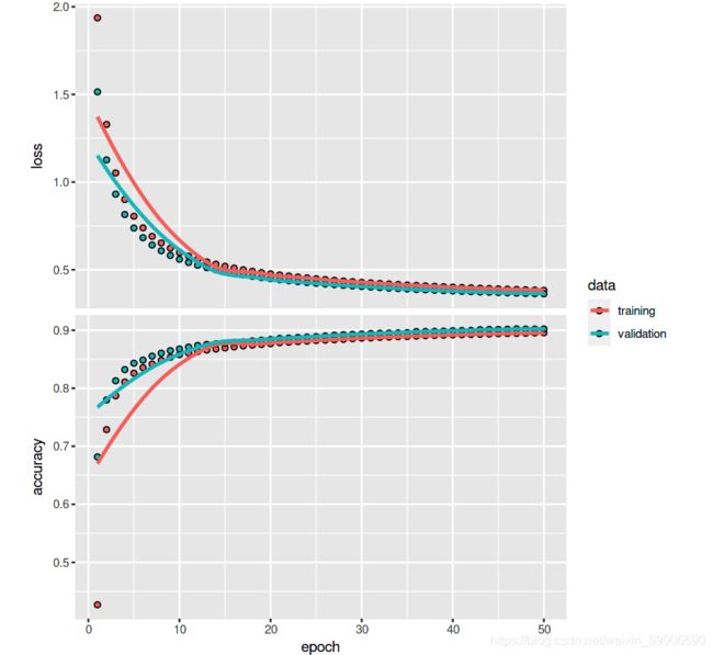
最后我们试试目前最先进之一的包Tensorflow里面的Keras模型框架来建造同样的Softmax回归模型，同时用的也是同样的数据和相同的周期。 结果是$90\%$左右，确实比我们的所写模型要优秀！

# ------------------------- Test the data on Keras ---------------------------
nn = keras_model_sequential()
nn %>%
  layer_dense(units = 10, input_shape = ncol(X_train_mat),
              activation = 'softmax')

nn %>% compile(
  loss = 'categorical_crossentropy',
  optimizer = 'sgd',
  metrics = c('accuracy')
)

history = nn %>% fit(
  X_train_mat, Y_train_oh, 
  epochs = 50, batch_size = 512,
  validation_data = list(X_test_mat, Y_test_oh)
)

plot(history)

总结下，虽然我们上面所实现的模型在速度和准确率上的确比不过目前大厂所研发的包（如Tensorflow， Mxnet等），但是通过一步一步的讲解和编码实现，希望能让有兴趣和刚入门的同学更好的了解到Softmax回归模型是如何解决分类问题和背后的数学公式是如何实现出来。最后值得一提的是，相信很多人都听说过或者使用过逻辑回归【logistic regression】，其实Softmax回归是逻辑回归的广泛版本。如果所遇到的分类问题只有两种分类目标的话（K=2），Softmax回归的假设函数和其它相关的公式会简化成逻辑回归的熟悉公式。有兴趣的同学可以自行推导一下看能不能得出逻辑回归的公式。