RNN, LSTM 图文详解

往期文章链接目录

Sequence Data

There are many sequence data in applications. Here are some examples

• Machine translation

  • from text sequence to text sequence.

• Text Summarization

  • from text sequence to text sequence.

• Sentiment classification

  • from text sequence to categories.

• Music Generation

  • from nothing or some simple stuff (character, integer, etc) to wave sequence.

• Name entity recognition (NER)

  • From text sequence to label sequence.

Why not use a standard neural network for sequence tasks

• Inputs, outputs can be different lengths in different examples. This can be solved by standard neural network by paddings with the maximum lengths but it’s not a good solution since there would be too many parameters.

• Doesn’t share features learned across different positions of text/sequence. Note that Convolutional Neural Network (CNN) is a good example of parameter sharing, so we should have a similar model for sequence data.

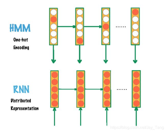
RNN

A Recurrent Neural Network (RNN) can be thought of as multiple copies of the same network, each passing a message to a successor. This chain-like nature reveals that recurrent neural networks are intimately related to sequences. Therefore, they’re the natural architecture of neural network to use for sequence data. Note that it also allows previous outputs to be used as inputs.

For each time step $t$, the activation $a^{<t>}$ and the output $y^{<t>}$ are expressed as follows:

• $a^{<t>}=g_1\left(W_{aa}{a}^{<t-1>}+W_{ax}{x}^{<t>}+b_a\right)$

• $y^{<t>}=g_2\left(W_{ya}{a}^{<t>}+b_y\right)$

These calculation could be visualized in the following figure

Note:

• dimension of $W_{aa}$: (number of hidden neurons, number of hidden neurons)

• dimension of $W_{ax}$: (number of hidden neurons, length of $x$)

• dimension of $W_{ya}$: (length of $y$, number of hidden neurons)

• The weight matrix $W_{aa}$ is the memory the RNN is trying to maintain from the previous layers.

• dimension of $b_a$: (number of hidden neurons, 1)

• dimension of $b_y$: (length of $y$, 1)

We can simplify the notations further;

• $a^{<t>}=g_1\left(W_a[a^{<t-1>},x^{<t>}]+b_a\right)$

• $y^{<t>}=g_2\left(W_y{a}^{<t>}+b_y\right)$

Note:

• $w_a$ is $w_{aa}$ and $w_{ax}$ stacked horizontally.

• $[a^{<t-1>},x^{<t>}]$ is $a^{<t-1>}$ and $x^{<t>}$ stacked vertically.

• dimension of $w_a$: (number of hidden neurons, number of hidden neurons $+$ length of $x$)

• dimension of $[a^{<t-1>},x^{<t>}]$: (number of hidden neurons $+$ length of $x$, 1)

Different types of RNNs

Loss function of RNN

The loss function $\mathcal{L}$ of all time steps is defined based on the loss at every time step as follows:

$$\mathcal{L}(\hat{y},y)=\sum _{t=1}^{T_y}\mathcal{L}\left({\hat{y}}^{<t>},y^{<t>}\right)$$

Backpropagation through time

Backpropagation is done at each point in time. At timestep $t$, the derivative of the loss
$\mathcal{L}$ with respect to weight matrix $W$ is expressed as follows:

$$\begin{array}{rlrl}\frac{\partial {\mathcal{L}}^{(t)}}{\partial W}& ={\sum _{k=0}^t\frac{\partial {\mathcal{L}}^{(t)}}{\partial W}|}_{(k)}& & \\ & =\sum _{k=0}^t\frac{\partial {\mathcal{L}}^{(t)}}{\partial y^{<t>}}\frac{\partial y^{<t>}}{\partial a^{<t>}}\frac{\partial a^{<t>}}{\partial a^{<k>}}\frac{\partial a^{<k>}}{\partial W}& & (1)\\ & =\sum _{k=0}^t\frac{\partial {\mathcal{L}}^{(t)}}{\partial y^{<t>}}\frac{\partial y^{<t>}}{\partial a^{<t>}}\left(\prod _{j=k+1}^t\frac{\partial a^{<j>}}{\partial a^{<j-1>}}\right)\frac{\partial a^{<k>}}{\partial W}& & (2)\end{array}$$

Note that from $(1)$ to $(2)$, we used the chain rule on $\frac{\partial a^{<t>}}{\partial a^{<k>}}$. From the derivative formula, we see that RNN could suffer from vanishing gradient descent problem easily.

Vanishing gradients with RNNs

Suppose we are working with language modeling problem and there are two sequences that model tries to learn:

• “The cat, which already ate …, was full”
• “The cats, which already ate …, were full”

The naive RNN is not very good at capturing very long-term dependencies like this. The reason is clear from the above section (Backpropagation through time).

Advantages and Drawbacks of RNN

Advantages:

• Possibility of processing input of any length.

• Model size not increasing with size of input.

• Computation takes into account historical information.

• Weights are shared across time.

Drawbacks:

• Computation being slow.

• Difficulty of accessing information from a long time ago.

• Cannot consider any future input for the current state.

LSTM

Long Short Term Memory (LSTM) networks are a special kind of RNN, capable of learning long-term dependencies. LSTMs are explicitly designed to avoid the long-term dependency problem. Remembering information for long periods of time is practically their default behavior, not something they struggle to learn.

Types of gates

In order to remedy the vanishing gradient problem, specific gates are used in some types of RNNs and usually have a well-defined purpose. They are usually noted $\Gamma$ and are equal to:

$$\Gamma =\sigma \left(W_1{a}^{<t-1>}+W_2{x}^{<t>}+b\right)$$

where $W_1,W_2,b$ are coefficients specific to the gate and $\sigma$ is the sigmoid function. We can also simplify it to

$$\Gamma =\sigma \left(W\left[a^{<t-1>},x^{<t>}\right]+b\right)$$

• Relevance gate ${\Gamma }_r$: Drop previous information?

• Forget gate ${\Gamma }_f$: Erase a cell or not?

• Output gate ${\Gamma }_o$: How much to reveal of a cell?

formulas and illustration of formulas

Variants of RNNs

Bi-directional RNN

• Part of the forward propagation goes from left to right, and part from right to left. Note that this is just a combination of two uni-directional RNN. It can’t strictly learn from “both sides”.

• To make predictions we use ${\hat{y}}^{<t>}$ by using the two activations that come from left and right.

• The blocks here can be any RNN block including the basic RNNs, LSTMs, or GRUs.

• The disadvantage of Bi-RNNs that you need the entire sequence before you can process it. For example, in live speech recognition if you use BiRNNs you will need to wait for the person who speaks to stop to take the entire sequence and then make your predictions.

Deep RNN

Note: In feed-forward deep nets, there could be $100$ or even $200$ layers. In deep RNNs stacking $3$ layers is already considered deep and expensive to train.

---

Reference:

• http://colah.github.io/posts/2015-08-Understanding-LSTMs/
• https://github.com/mbadry1/DeepLearning.ai-Summary/tree/master/5-%20Sequence%20Models#recurrent-neural-networks
• https://stanford.edu/~shervine/teaching/cs-230/cheatsheet-recurrent-neural-networks

往期文章链接目录