深度学习Day-41:使用Word2vec实现文本分类
本文为:[365天深度学习训练营] 中的学习记录博客
原作者:[K同学啊 | 接辅导、项目定制]
任务:
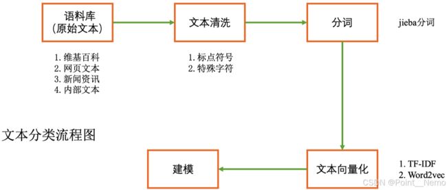
本次将加入Word2vec使用PyTorch实现中文文本分类,Word2Vec 则是其中的一种词嵌入方法,是一种用于生成词向量的浅层神经网络模型,由Tomas Mikolov及其团队于2013年提出。Word2Vec通过学习大量文本数据,将每个单词表示为一个连续的向量,这些向量可以捕捉单词之间的语义和句法关系。数据示例如下:

- 结合Word2Vec文本内容(第1列)预测文本标签(第2列)
- 优化本文网络结构,将准确率提升至89%
- 绘制出验证集的ACC与Loss图
进阶:
- 尝试根据第2周的内容独立实现,尽可能的不看本文的代码
1. 加载数据
import torch
import warnings

warnings.filterwarnings("ignore")             #忽略警告信息

# win10系统
device = torch.device("cuda" if torch.cuda.is_available() else "cpu")
print(device)
代码输出为:
cpu接着,运行下面代码:
import pandas as pd

# 加载自定义中文数据
train_data = pd.read_csv('data/train.csv', sep='\t', header=None)
train_data.head()
代码输出为:
                       0              1
0      还有双鸭山到淮阴的汽车票吗13号的   Travel-Query
1                从这里怎么回家   Travel-Query
2       随便播放一首专辑阁楼里的佛里的歌     Music-Play
3              给看一下墓王之王嘛  FilmTele-Play
4  我想看挑战两把s686打突变团竞的游戏视频     Video-Play
接着,运行下面代码:
# 构造数据集迭代器
def coustom_data_iter(texts, labels):
    for x, y in zip(texts, labels):
        yield x, y

x = train_data[0].values[:]
# 多类标签的one-hot展开
y = train_data[1].values[:]
print(x)
print(y)
代码输出为:
['还有双鸭山到淮阴的汽车票吗13号的' '从这里怎么回家' '随便播放一首专辑阁楼里的佛里的歌' ...
 '黎耀祥陈豪邓萃雯畲诗曼陈法拉敖嘉年杨怡马浚伟等到场出席' '百事盖世群星星光演唱会有谁' '下周一视频会议的闹钟帮我开开']
['Travel-Query' 'Travel-Query' 'Music-Play' ... 'Radio-Listen'
 'Video-Play' 'Alarm-Update']
zip 是 Python 中的一个内置函数,它可以将多个序列(列表、元组等)中对应的元素打包成一个个元组,然后返回这些元组组成的一个迭代器。例如,在代码中 zip(texts, labels) 就是将 texts 和 labels 两个列表中对应位置的元素一一打包成元组,返回一个迭代器,每次迭代返回一个元组 (x, y),其中 x 是 texts 中的一个元素,y 是 labels 中对应的一个元素。这样,每次从迭代器中获取一个元素,就相当于从 texts 和 labels 中获取了一组对应的数据。在这里,zip 函数主要用于将输入的 texts 和 labels 打包成一个可迭代的数据集,然后传给后续的模型训练过程使用。
2. 构建词典
from gensim.models.word2vec import Word2Vec
import numpy as np

# 训练 Word2Vec 浅层神经网络模型
w2v = Word2Vec(vector_size=100, #是指特征向量的维度,默认为100。
               min_count=3)     #可以对字典做截断. 词频少于min_count次数的单词会被丢弃掉, 默认值为5。

w2v.build_vocab(x)
w2v.train(x,
          total_examples=w2v.corpus_count,
          epochs=20)
Word2Vec可以直接训练模型,一步到位。这里分了三步:
- 构建一个空模型。
- build_vocab 方法根据输入的文本数据 x 构建词典。build_vocab 方法会统计输入文本中每个词汇出现的次数,并按照词频从高到低的顺序将词汇加入词典中。
- 使用 train 方法对模型进行训练,total_examples 参数指定了训练时使用的文本数量,这里使用的是 w2v.corpus_count 属性,表示输入文本的数量。
如果一步到位的话代码为:
w2v = Word2Vec(x, vector_size=100, min_count=3, epochs=20)
print(w2v)
代码输出为:
Word2Vec接着,运行代码:
# 将文本转化为向量
def average_vec(text):
    vec = np.zeros(100).reshape((1, 100))
    for word in text:
        try:
            vec += w2v.wv[word].reshape((1, 100))
        except KeyError:
            continue
    return vec

# 将词向量保存为 Ndarray
x_vec = np.concatenate([average_vec(z) for z in x])

# 保存 Word2Vec 模型及词向量
w2v.save('w2v_model.pkl')
train_iter = coustom_data_iter(x_vec, y)
print(len(x),len(x_vec))
代码输出为:
12100 12100这段代码定义了一个函数 average_vec(text),它接受一个包含多个词的列表 text 作为输入,并返回这些词对应词向量的平均值。该函数:
- 初始化一个形状为 (1, 100) 的全零 numpy 数组来表示平均向量
- 遍历 text 中的每个词,并尝试从 Word2Vec 模型 w2v 中使用 wv 属性获取其对应的词向量。如果在模型中找到了该词,函数将其向量加到 vec中。如果未找到该词,函数会继续迭代下一个词
- 函数返回平均向量 vec
然后使用列表推导式将 average_vec() 函数应用于列表 x 中的每个元素。得到的平均向量列表使用 np.concatenate() 连接成一个 numpy 数组 x_vec,该数组表示 x 中所有元素的平均向量。x_vec 的形状为 (n, 100),其中 n 是 x 中元素的数量。
接着,运行代码:
label_name = list(set(train_data[1].values[:]))
print(label_name)
代码输出为:
['Radio-Listen', 'Music-Play', 'Audio-Play', 'Calendar-Query', 'Video-Play', 'Other', 'HomeAppliance-Control', 'Alarm-Update', 'TVProgram-Play', 'FilmTele-Play', 'Weather-Query', 'Travel-Query']
3.生成数据批次和迭代器
text_pipeline  = lambda x: average_vec(x)
label_pipeline = lambda x: label_name.index(x)

print(text_pipeline("你在干嘛"))
print(label_pipeline("Travel-Query"))
代码输出为:
[[-0.50475422  1.40358877  2.10718489  0.62696353 -2.27326742 -0.86325586
   1.91590985  0.02256403  0.70883784 -0.45788445 -1.81392689 -4.50311214
   1.78359316 -0.25500346 -0.56241548  0.44832698  3.47105673 -2.67846954
   3.39968163 -1.39780461  2.82882937 -1.61015151  0.25089827 -0.07058875
  -0.4996658  -1.54310556 -1.56648542 -1.26974761  1.67414579 -0.96915421
   2.55048783  1.92456639 -0.48464253 -0.32199331 -0.30795002  0.3949365
  -0.14144704  4.1541061  -0.9569176   1.55245852 -0.4631255   0.88437843
  -0.58941404  1.80091982  0.012504    0.66884801  1.86418419 -0.68803712
  -2.61692403  2.41418719  0.92531049 -2.14762762 -1.14705408 -0.94946782
  -0.43397234 -0.83550627  1.14806312 -0.48897886 -0.26805569  0.28821549
   0.59152652 -1.84648283  3.38585148 -0.64367552 -0.29464381 -0.25962844
  -1.39986839  1.29020444  0.3520185  -0.11786325  0.61111923  0.30863122
   1.81852724 -0.88515008  0.20038423 -0.88415289 -3.15321362  0.56210989
   1.42266002  0.29345044 -1.37240933 -0.26137188 -2.56611562  2.25422826
  -2.40777135 -1.40590963  1.56099287 -2.09348607 -0.59971704  0.03473149
  -0.39137083 -0.15937868  1.691751    1.63441243  0.41640663 -1.43600623
  -1.06085297  0.74154633 -1.4142051   0.06242213]]
11
lambda 表达式的语法为:lambda arguments: expression
其中 arguments 是函数的参数,可以有多个参数,用逗号分隔。expression 是一个表达式,它定义了函数的返回值。
- text_pipeline 函数:接受一个包含多个词的列表 x 作为输入,并返回这些词对应词向量的平均值,即调用了之前定义的 average_vec 函数。这个函数用于将原始文本数据转换为词向量平均值表示的形式
- label_pipeline 函数:接受一个标签名 x 作为输入,并返回该标签名label_name 列表中的索引。这个函数可以用于将原始标签数据转换为数字索引表示的形式
接着运行:
vocab(['我','想','看','和平','精英','上','战神','必备','技巧','的','游戏','视频'])
label_name = list(set(train_data[1].values[:]))
print(label_name)
代码输出为:
['Radio-Listen', 'Travel-Query', 'HomeAppliance-Control', 'Other', 'Audio-Play', 'Calendar-Query', 'Weather-Query', 'FilmTele-Play', 'TVProgram-Play', 'Alarm-Update', 'Music-Play', 'Video-Play']接着运行:
text_pipeline  = lambda x: vocab(tokenizer(x))
label_pipeline = lambda x: label_name.index(x)

print(text_pipeline('我想看和平精英上战神必备技巧的游戏视频'))
print(label_pipeline('Video-Play'))
代码输出为:
[2, 10, 13, 973, 1079, 146, 7724, 7574, 7793, 1, 186, 28]
11
ambda 表达式的语法为:lambda arguments: expression
其中 arguments 是函数的参数,可以有多个参数,用逗号分隔。expression 是一个表达式,它定义了函数的返回值。
- text_pipeline函数:将原始文本数据转换为整数列表,使用了之前构建的vocab词表和tokenizer分词器函数。具体来说,它接受一个字符串x作为输入,首先使用tokenizer将其分词,然后将每个词在vocab词表中的索引放入一个列表中返回。
- label_pipeline函数:将原始标签数据转换为整数,它接受一个字符串x作为输入,并使用label_name.index(x)方法获取 x 在 label_name 列表中的索引作为输出。
接着,运行下面代码:
from torch.utils.data import DataLoader

def collate_batch(batch):
    label_list, text_list = [], []

    for (_text, _label) in batch:
        # 标签列表
        label_list.append(label_pipeline(_label))

        # 文本列表
        processed_text = torch.tensor(text_pipeline(_text), dtype=torch.float32)
        text_list.append(processed_text)

    label_list = torch.tensor(label_list, dtype=torch.int64)
    text_list = torch.cat(text_list)

    return text_list.to(device), label_list.to(device)

# 数据加载器,调用示例
dataloader = DataLoader(train_iter,
                        batch_size=8,
                        shuffle=False,
                        collate_fn=collate_batch)
4.模型构建
4.1 搭建模型
from torch import nn

class TextClassificationModel(nn.Module):

    def __init__(self, num_class):
        super(TextClassificationModel, self).__init__()
        self.fc = nn.Linear(100, num_class)

    def forward(self, text):
        return self.fc(text)
4.2 初始化模型
num_class  = len(label_name)
vocab_size = 100000
em_size    = 12
model      = TextClassificationModel(num_class).to(device)
4.3 定义训练函数与评估函数
import time

def train(dataloader):
    model.train()  # 切换为训练模式
    total_acc, train_loss, total_count = 0, 0, 0
    log_interval = 50
    start_time = time.time()

    for idx, (text, label) in enumerate(dataloader):
        predicted_label = model(text)

        optimizer.zero_grad()  # grad属性归零
        loss = criterion(predicted_label, label)  # 计算网络输出和真实值之间的差距,label为真实值
        loss.backward()  # 反向传播
        torch.nn.utils.clip_grad_norm_(model.parameters(), 0.1)  # 梯度裁剪
        optimizer.step()  # 每一步自动更新

        # 记录acc与loss
        total_acc += (predicted_label.argmax(1) == label).sum().item()
        train_loss += loss.item()
        total_count += label.size(0)

        if idx % log_interval == 0 and idx > 0:
            elapsed = time.time() - start_time
            print('| epoch {:1d} | {:4d}/{:4d} batches '
                  '| train_acc {:4.3f} train_loss {:4.5f}'.format(epoch, idx, len(dataloader),
                                                                  total_acc / total_count, train_loss / total_count))
            total_acc, train_loss, total_count = 0, 0, 0
            start_time = time.time()


def evaluate(dataloader):
    model.eval()  # 切换为测试模式
    total_acc, train_loss, total_count = 0, 0, 0

    with torch.no_grad():
        for idx, (text, label) in enumerate(dataloader):
            predicted_label = model(text)

            loss = criterion(predicted_label, label)  # 计算loss值
            # 记录测试数据
            total_acc += (predicted_label.argmax(1) == label).sum().item()
            train_loss += loss.item()
            total_count += label.size(0)

    return total_acc / total_count, train_loss / total_count
torch.nn.utils.clip_grad_norm_(model.parameters(), 0.1)是一个PyTorch函数,用于在训练神经网络时限制梯度的大小。这种操作被称为梯度裁剪(gradient clipping),可以防止梯度爆炸问题,从而提高神经网络的稳定性和性能。
在这个函数中:
- model.parameters()表示模型的所有参数。对于一个神经网络,参数通常包括权重和偏置项。
- 0.1是一个指定的阈值,表示梯度的最大范数(L2范数)。如果计算出的梯度范数超过这个阈值,梯度会被缩放,使其范数等于阈值。
梯度裁剪的主要目的是防止梯度爆炸。梯度爆炸通常发生在训练深度神经网络时,尤其是在处理长序列数据的循环神经网络(RNN)中。当梯度爆炸时,参数更新可能会变得非常大,导致模型无法收敛或出现数值不稳定。通过限制梯度的大小,梯度裁剪有助于解决这些问题,使模型训练变得更加稳定。
5.训练模型
5.1 拆分数据集并运行模型
from torch.utils.data.dataset import random_split
from torchtext.data.functional import to_map_style_dataset

# 超参数
EPOCHS = 10  # epoch
LR = 5  # 学习率
BATCH_SIZE = 64  # batch size for training

criterion = torch.nn.CrossEntropyLoss()
optimizer = torch.optim.SGD(model.parameters(), lr=LR)
scheduler = torch.optim.lr_scheduler.StepLR(optimizer, 1.0, gamma=0.1)
total_accu = None

# 构建数据集
train_iter = coustom_data_iter(train_data[0].values[:], train_data[1].values[:])
train_dataset = to_map_style_dataset(train_iter)

split_train_, split_valid_ = random_split(train_dataset,
                                          [int(len(train_dataset) * 0.8), int(len(train_dataset) * 0.2)])

train_dataloader = DataLoader(split_train_, batch_size=BATCH_SIZE,
                              shuffle=True, collate_fn=collate_batch)

valid_dataloader = DataLoader(split_valid_, batch_size=BATCH_SIZE,
                              shuffle=True, collate_fn=collate_batch)

total_val_acc = []
total_val_loss = []

# best_val_acc = 0    # 设置一个最佳准确率,作为最佳模型的判别指标

for epoch in range(1, EPOCHS + 1):
    epoch_start_time = time.time()
    train(train_dataloader)
    val_acc, val_loss = evaluate(valid_dataloader)

    # 保存最佳模型到 best_model
    # if val_acc > best_val_acc:
    #     best_val_acc   = val_acc
    #     best_model = copy.deepcopy(model)

    total_val_acc.append(val_acc)
    total_val_loss.append(val_loss)

    # 获取当前的学习率
    lr = optimizer.state_dict()['param_groups'][0]['lr']

    if total_accu is not None and total_accu > val_acc:
        scheduler.step()
    else:
        total_accu = val_acc

    print('-' * 69)
    print('| epoch {:1d} | time: {:4.2f}s | '
          'valid_acc {:4.3f} valid_loss {:4.3f} | lr {:4.6f}'.format(epoch,
                                                                     time.time() - epoch_start_time,
                                                                     val_acc, val_loss, lr))

    print('-' * 69)
代码输出为:
| epoch 1 |   50/ 152 batches | train_acc 0.752 train_loss 0.02407
| epoch 1 |  100/ 152 batches | train_acc 0.822 train_loss 0.01892
| epoch 1 |  150/ 152 batches | train_acc 0.830 train_loss 0.01872
---------------------------------------------------------------------
| epoch 1 | time: 0.71s | valid_acc 0.858 valid_loss 0.014 | lr 5.000000
---------------------------------------------------------------------
| epoch 2 |   50/ 152 batches | train_acc 0.850 train_loss 0.01587
| epoch 2 |  100/ 152 batches | train_acc 0.844 train_loss 0.01787
| epoch 2 |  150/ 152 batches | train_acc 0.839 train_loss 0.01798
---------------------------------------------------------------------
| epoch 2 | time: 0.73s | valid_acc 0.852 valid_loss 0.021 | lr 5.000000
---------------------------------------------------------------------
| epoch 3 |   50/ 152 batches | train_acc 0.884 train_loss 0.01207
| epoch 3 |  100/ 152 batches | train_acc 0.894 train_loss 0.00914
| epoch 3 |  150/ 152 batches | train_acc 0.896 train_loss 0.00819
---------------------------------------------------------------------
| epoch 3 | time: 0.84s | valid_acc 0.887 valid_loss 0.010 | lr 0.500000
---------------------------------------------------------------------
| epoch 4 |   50/ 152 batches | train_acc 0.902 train_loss 0.00737
| epoch 4 |  100/ 152 batches | train_acc 0.891 train_loss 0.00707
| epoch 4 |  150/ 152 batches | train_acc 0.895 train_loss 0.00737
---------------------------------------------------------------------
| epoch 4 | time: 0.70s | valid_acc 0.887 valid_loss 0.009 | lr 0.500000
---------------------------------------------------------------------
| epoch 5 |   50/ 152 batches | train_acc 0.894 train_loss 0.00665
| epoch 5 |  100/ 152 batches | train_acc 0.900 train_loss 0.00636
| epoch 5 |  150/ 152 batches | train_acc 0.900 train_loss 0.00642
---------------------------------------------------------------------
| epoch 5 | time: 0.68s | valid_acc 0.880 valid_loss 0.009 | lr 0.500000
---------------------------------------------------------------------
| epoch 6 |   50/ 152 batches | train_acc 0.904 train_loss 0.00613
| epoch 6 |  100/ 152 batches | train_acc 0.913 train_loss 0.00541
| epoch 6 |  150/ 152 batches | train_acc 0.906 train_loss 0.00583
---------------------------------------------------------------------
| epoch 6 | time: 0.67s | valid_acc 0.890 valid_loss 0.008 | lr 0.050000
---------------------------------------------------------------------
| epoch 7 |   50/ 152 batches | train_acc 0.914 train_loss 0.00521
| epoch 7 |  100/ 152 batches | train_acc 0.907 train_loss 0.00587
| epoch 7 |  150/ 152 batches | train_acc 0.902 train_loss 0.00569
---------------------------------------------------------------------
| epoch 7 | time: 0.69s | valid_acc 0.891 valid_loss 0.008 | lr 0.050000
---------------------------------------------------------------------
| epoch 8 |   50/ 152 batches | train_acc 0.909 train_loss 0.00560
| epoch 8 |  100/ 152 batches | train_acc 0.907 train_loss 0.00571
| epoch 8 |  150/ 152 batches | train_acc 0.908 train_loss 0.00519
---------------------------------------------------------------------
| epoch 8 | time: 0.69s | valid_acc 0.890 valid_loss 0.008 | lr 0.050000
---------------------------------------------------------------------
| epoch 9 |   50/ 152 batches | train_acc 0.907 train_loss 0.00572
| epoch 9 |  100/ 152 batches | train_acc 0.908 train_loss 0.00531
| epoch 9 |  150/ 152 batches | train_acc 0.907 train_loss 0.00523
---------------------------------------------------------------------
| epoch 9 | time: 0.66s | valid_acc 0.889 valid_loss 0.008 | lr 0.005000
---------------------------------------------------------------------
| epoch 10 |   50/ 152 batches | train_acc 0.900 train_loss 0.00576
| epoch 10 |  100/ 152 batches | train_acc 0.915 train_loss 0.00501
| epoch 10 |  150/ 152 batches | train_acc 0.911 train_loss 0.00546
---------------------------------------------------------------------
| epoch 10 | time: 1.14s | valid_acc 0.889 valid_loss 0.008 | lr 0.000500
---------------------------------------------------------------------
torch.Size([1, 100])
该文本的类别是:Travel-Query

Process finished with exit code 0
接着运行下述代码:
test_acc, test_loss = evaluate(valid_dataloader)
print('模型准确率为:{:5.4f}'.format(test_acc))
代码输出为:
模型准确率为:0.88315.2 使用测试数据集评估模型
def predict(text, text_pipeline):
    with torch.no_grad():
        text = torch.tensor(text_pipeline(text), dtype=torch.float32)
        print(text.shape)
        output = model(text)
        return output.argmax(1).item()

ex_text_str = "还有双鸭山到淮阴的汽车票吗13号的"

model = model.to("cpu")

print("该文本的类别是:%s" %label_name[predict(ex_text_str, text_pipeline)])
代码输出为:
torch.Size([1, 100])
该文本的类别是:Travel-Query
5.3 结果可视化
import matplotlib.pyplot as plt
#隐藏警告
import warnings
warnings.filterwarnings("ignore")               #忽略警告信息
plt.rcParams['font.sans-serif']    = ['SimHei'] # 用来正常显示中文标签
plt.rcParams['axes.unicode_minus'] = False      # 用来正常显示负号
plt.rcParams['figure.dpi']         = 100        #分辨率

epochs_range = range(EPOCHS)

plt.figure(figsize=(12, 3))
plt.subplot(1, 2, 1)

plt.plot(epochs_range, total_val_acc, label='Val Accuracy')
plt.legend(loc='lower right')
plt.title('Validation Accuracy')

plt.subplot(1, 2, 2)
plt.plot(epochs_range, total_val_loss, label='Val Loss')
plt.legend(loc='upper right')
plt.title('Validation Loss')
plt.show()
可视化结果:
