ubuntu22.04@laptop OpenCV Get Started: 015_deep_learning_with_opencv_dnn_module

1. 源由

计算机视觉领域自20世纪60年代末以来就存在。图像分类和物体检测是计算机视觉中一些最古老的问题，研究人员尝试解决这些问题已经数十年。

目前，使用神经网络和深度学习，已经达到了一个阶段，计算机可以开始以高精度实际理解和识别对象，甚至在许多情况下超过人类。

要了解有关神经网络和深度学习与计算机视觉的知识，OpenCV DNN 模块是一个很好的起点。由于其高度优化的 CPU 性能，即使没有非常强大的GPU，初学者也可以轻松体验。

2. 应用Demo

015_deep_learning_with_opencv_dnn_module是基于OpenCV DNN的物体分类和物体检测的示例程序。

2.1 C++应用Demo

C++应用Demo工程结构：

015_deep_learning_with_opencv_dnn_module/CPP$ tree .
.
├── classify
│   ├── classify.cpp
│   └── CMakeLists.txt
└── detection
    ├── detect_img
    │   ├── CMakeLists.txt
    │   └── detect_img.cpp
    └── detect_vid
        ├── CMakeLists.txt
        └── detect_vid.cpp

4 directories, 6 files

确认OpenCV安装路径：

$ find /home/daniel/ -name "OpenCVConfig.cmake"
/home/daniel/OpenCV/installation/opencv-4.9.0/lib/cmake/opencv4/
/home/daniel/OpenCV/opencv/build/OpenCVConfig.cmake
/home/daniel/OpenCV/opencv/build/unix-install/OpenCVConfig.cmake


$ export OpenCV_DIR=/home/daniel/OpenCV/installation/opencv-4.9.0/lib/cmake/opencv4/

C++应用Demo工程编译执行：

$ cd classify
$ mkdir build
$ cd build
$ cmake ..
$ cmake --build . --config Release
$ cd ..
$ ./build/classify

$ cd detection/detect_img
$ mkdir build
$ cd build
$ cmake ..
$ cmake --build . --config Release
$ cd ..
$ ./build/detect_img

$ cd detection/detect_vid
$ mkdir build
$ cd build
$ cmake ..
$ cmake --build . --config Release
$ cd ..
$ ./build/detect_vid

2.2 Python应用Demo

Python应用Demo工程结构：

015_deep_learning_with_opencv_dnn_module/Python$ tree .
.
├── classification
│   └── classify.py
├── detection
│   ├── detect_img.py
│   └── detect_vid.py
└── requirements.txt

2 directories, 4 files

Python应用Demo工程执行：

$ workoncv-4.9.0
$ cd classification
$ python classify.py
$ cd ..
$ cd detection
$ python detect_img.py
$ python detect_vid.py

3. 使用 OpenCV DNN 模块进行图像分类

我们将使用在非常著名的 ImageNet 数据集上使用 Caffe 框架训练的神经网络模型。

具体来说，我们将使用 DensNet121 深度神经网络模型进行分类任务。其优势在于它在 ImageNet 数据集的 1000 个类别上进行了预训练。我们可以期望该模型已经见过我们想要分类的任何图像。这使我们可以从一个广泛的图像范围中进行选择。

以下是对图像进行分类时将遵循的步骤：

1. 从磁盘加载类名文本文件并提取所需的标签。
2. 从磁盘加载预训练的神经网络模型。
3. 从磁盘加载图像并准备图像，使其符合深度学习模型的正确输入格式。
4. 将输入图像通过模型进行前向传播，并获取输出。
5. 将获取的输出数据，分析后标记识别物体输出。

3.1 导入模块并加载类名文本文件

我们将使用的 DenseNet121 模型是在 1000 个 ImageNet 类别上进行训练的。我们需要一种方式将这 1000 个类别加载到内存中，并且能够轻松地访问它们。这些类别通常以文本文件的形式提供。其中一个文件称为 classification_classes_ILSVRC2012.txt，其中以以下格式包含所有类别的名称。

tench, Tinca tinca
goldfish, Carassius auratus
great white shark, white shark, man-eater, man-eating shark, Carcharodon carcharias
tiger shark, Galeocerdo cuvieri
hammerhead, hammerhead shark

每一行包含了与单个图像相关的所有标签或类名。例如，第一行包含了 tench 和 Tinca Tinca。这两个名称都属于同一种鱼类。类似地，第二行有两个属于金鱼的名称。通常，第一个名称是几乎所有人都能认识的最常见的名称。

C++:

    std::vector class_names;
    ifstream ifs(string("../../input/classification_classes_ILSVRC2012.txt").c_str());
    string line;
    while (getline(ifs, line))
    {
        class_names.push_back(line);
    } 

Python:

# read the ImageNet class names
with open('../../input/classification_classes_ILSVRC2012.txt', 'r') as f:
    image_net_names = f.read().split('\n')
# final class names (just the first word of the many ImageNet names for one image)
class_names = [name.split(',')[0] for name in image_net_names]

3.2 从磁盘加载预训练 DenseNet121 模型

正如之前讨论的，我们将使用一个使用 Caffe 深度学习框架进行训练的预训练 DenseNet121 模型。

我们将需要模型权重文件（.caffemodel）和模型配置文件（.prototxt）。

C++:

    // load the neural network model
    auto model = readNet("../../input/DenseNet_121.prototxt", 
                        "../../input/DenseNet_121.caffemodel", 
                        "Caffe");

Python:

# load the neural network model
model = cv2.dnn.readNet(model='../../input/DenseNet_121.caffemodel', 
                      config='../../input/DenseNet_121.prototxt', 
                      framework='Caffe')

通过使用 OpenCV DNN 模块中的 readNet() 函数加载模型，该函数接受三个输入参数。

• model: 这是预训练权重文件的路径。在我们的情况下，它是预训练的 Caffe 模型。
• config: 这是模型配置文件的路径，在这种情况下是 Caffe 模型的 .prototxt 文件。
• framework: 最后，我们需要提供我们加载模型的框架名称。对于我们来说，它是 Caffe 框架。

3.3 读取图像并准备为模型输入

我们将像往常一样使用 OpenCV 的 imread() 函数从磁盘读取图像。请注意，需要处理一些其他细节：使用 DNN 模块加载的预训练模型不会直接将读取的图像作为输入。

C++:

    // load the image from disk
    Mat image = imread("../../input/image_1.jpg");
    // create blob from image
    Mat blob = blobFromImage(image, 0.01, Size(224, 224), Scalar(104, 117, 123));

Python:

# load the image from disk
image = cv2.imread('../../input/image_1.jpg')
# create blob from image
blob = cv2.dnn.blobFromImage(image=image, scalefactor=0.01, size=(224, 224), 
                             mean=(104, 117, 123))

在读取图像时，我们假设它位于当前目录的上两级目录，并在 input 文件夹内。接下来的几个步骤非常重要，有一个 blobFromImage() 函数，它将图像准备成正确的格式以输入模型。让我们详细了解一下所有参数。

• image: 这是我们刚刚使用 imread() 函数读取的输入图像。
• scalefactor: 这个值按照提供的值对图像进行缩放。它有一个默认值为1，表示不进行缩放。
• size: 这是图像将被调整到的大小。我们提供的大小为 224×224，因为大多数在 ImageNet 数据集上训练的分类模型都希望输入的大小是这个尺寸。
• mean: mean 参数非常重要。这实际上是从图像的 RGB 色道中减去的平均值。这样做可以对输入进行标准化，并使最终的输入对不同的光照尺度具有不变性。

还有一件事需要注意。所有深度学习模型都期望以批量形式输入。然而，在这里我们只有一张图像。尽管如此，blobFromImage() 函数产生的 blob 输出实际上具有 [1, 3, 224, 224] 的形状。请注意，blobFromImage() 函数添加了一个额外的批量维度。这将是神经网络模型的最终和正确的输入格式。

3.4 通过模型进行前向传播

进行预测有两个步骤。

1. 将输入 blob 设置为我们从磁盘加载的神经网络模型。
2. 使用 forward() 函数将 blob 通过模型进行前向传播，这将给出所有的输出。

C++:

    // set the input blob for the neural network
    model.setInput(blob);
    // forward pass the image blob through the model
    Mat outputs = model.forward();

Python:

# set the input blob for the neural network
model.setInput(blob)
# forward pass image blog through the model
outputs = model.forward()

3.5 数据分析及标记输出

输出是一个数组，保存了所有的预测结果。但在我们能够正确地查看输出和类标签之前，还需要完成一些预处理步骤。

[[-1.44623446e+00]
[-6.37421310e-01]
[-1.04836571e+00]
[-8.40160131e-01]
…
]

当前，输出的形状为 (1, 1000, 1, 1)，如果保持这样的形状，提取类标签会比较困难。因此，下面的代码块重新调整了输出的形状，然后我们可以轻松地获取正确的类标签，并将标签 ID 映射到类名。

C++:

    Point classIdPoint;
    double final_prob;
    minMaxLoc(outputs.reshape(1, 1), 0, &final_prob, 0, &classIdPoint);
    int label_id = classIdPoint.x;

    // Print predicted class.
    string out_text = format("%s, %.3f", (class_names[label_id].c_str()), final_prob);
    // put the class name text on top of the image
    putText(image, out_text, Point(25, 50), FONT_HERSHEY_SIMPLEX, 1, Scalar(0, 255, 0),
                2);
        
    imshow("Image", image);
    imwrite("../../outputs/result_image.jpg", image);

Python:

final_outputs = outputs[0]
# make all the outputs 1D
final_outputs = final_outputs.reshape(1000, 1)
# get the class label
label_id = np.argmax(final_outputs)
# convert the output scores to softmax probabilities
probs = np.exp(final_outputs) / np.sum(np.exp(final_outputs))
# get the final highest probability
final_prob = np.max(probs) * 100.
# map the max confidence to the class label names
out_name = class_names[label_id]
out_text = f"{out_name}, {final_prob:.3f}"

# put the class name text on top of the image
cv2.putText(image, out_text, (25, 50), cv2.FONT_HERSHEY_SIMPLEX, 1, (0, 255, 0),
            2)
cv2.imshow('Image', image)
cv2.waitKey(0)
cv2.imwrite('../../outputs/result_image.jpg', image)

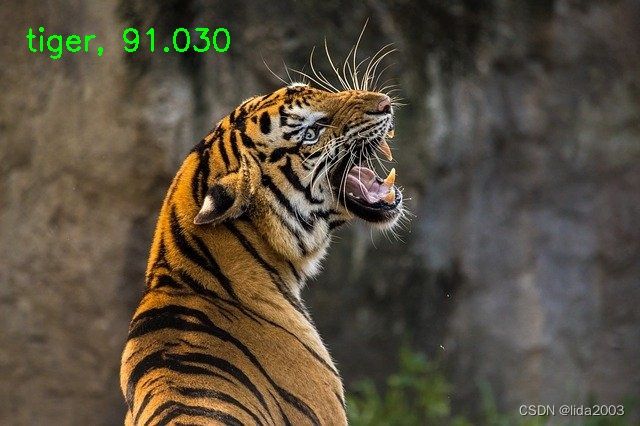
3.6 效果

DenseNet121 模型准确地将图像预测为一只老虎，且置信度达到了 91%。结果相当不错。

4. 使用 OpenCV DNN 模块进行目标检测

使用 OpenCV DNN 模块，可以轻松地开始深度学习和计算机视觉中的目标检测任务。与分类任务类似，我们将加载图像、适当的模型，并将输入通过模型进行前向传播。然而，用于目标检测的预处理步骤与分类任务有所不同，这是因为在目标检测中，我们通常需要在图像上绘制检测到的对象的边界框和类别标签。

4.1 使用 OpenCV DNN 进行图像目标检测

就像分类任务一样，我们在这里也将利用预训练模型。这些模型是在 MS COCO 数据集上进行训练的，这是当前基于深度学习的目标检测模型的基准数据集。

MS COCO 数据集包含几乎 80 类对象，从人到汽车再到牙刷等各种日常物品。该数据集包含 80 种常见物体的类别。我们还将使用一个文本文件来加载 MS COCO 数据集中所有对象检测标签。

我们将使用 MobileNet SSD（Single Shot Detector），该模型是使用 TensorFlow 深度学习框架在 MS COCO 数据集上进行训练的。SSD 模型通常比其他目标检测模型更快。此外，MobileNet 的骨干网络还使它们的计算量更少。因此，使用 OpenCV DNN 学习目标检测的一个好的起点是使用 MobileNet SSD 模型。

4.1.1 导入模块并加载类名文本文件

接下来我们读取名为 object_detection_classes_coco.txt 的文件，其中包含所有类别名称，每个名称都由换行符分隔。我们将每个类别名称存储在 class_names 列表中。

class_names 列表将类似于以下内容。

[‘person’, ‘bicycle’, ‘car’, ‘motorcycle’, ‘airplane’, ‘bus’, ‘train’, ‘truck’, ‘boat’, ‘traffic light’, … ‘book’, ‘clock’, ‘vase’, ‘scissors’, ‘teddy bear’, ‘hair drier’, ‘toothbrush’, ‘’]

C++:

    std::vector class_names;
    ifstream ifs(string("../../../input/object_detection_classes_coco.txt").c_str());
    string line;
    while (getline(ifs, line))
    {
        class_names.push_back(line);
    }  

Python:

# load the COCO class names
with open('../../input/object_detection_classes_coco.txt', 'r') as f:
    class_names = f.read().split('\n')

# get a different color array for each of the classes
COLORS = np.random.uniform(0, 255, size=(len(class_names), 3))

4.1.2 从磁盘加载预训练 MobileNet SSD 模型

model参数接受推理文件路径作为输入，这是一个包含权重的预训练模型。
config参数接受模型配置文件的路径，这是一个Protobuf文本文件。
最后，指定了框架是TensorFlow。

C++:

    // load the neural network model
    auto model = readNet("../../../input/frozen_inference_graph.pb", 
                        "../../../input/ssd_mobilenet_v2_coco_2018_03_29.pbtxt.txt", 
                        "TensorFlow");

Python:

# load the DNN model
model = cv2.dnn.readNet(model='../../input/frozen_inference_graph.pb',
                        config='../../input/ssd_mobilenet_v2_coco_2018_03_29.pbtxt.txt', 
                        framework='TensorFlow')

4.1.3 读取图像并前向传播

对于目标检测，我们在blobFromImage()函数中使用了略有不同的参数值。

指定大小为300×300，这是SSD模型几乎所有框架通常期望的输入大小。TensorFlow也是如此。

还使用了swapRB参数。通常，OpenCV以BGR格式读取图像，而目标检测模型期望输入为RGB格式。因此，swapRB参数将交换图像的R和B通道，使其成为RGB格式。

然后，将blob设置为MobileNet SSD模型，并使用forward()函数进行前向传播。

输出结构如下：

[[[[0.00000000e+00 1.00000000e+00 9.72869813e-01 2.06566155e-02 1.11088693e-01 2.40461200e-01 7.53399074e-01]]]]

• 索引位置1包含类别标签，其取值范围可以从1到80。
• 索引位置2包含置信度分数。这不是概率分数，而是模型对其检测到的属于某个类别的对象的置信度。
• 最后四个值中，前两个是x、y边界框坐标，最后一个是边界框的宽度和高度。

C++:

    // read the image from disk
    Mat image = imread("../../../input/image_2.jpg");
    int image_height = image.cols;
    int image_width = image.rows;
    //create blob from image
    Mat blob = blobFromImage(image, 1.0, Size(300, 300), Scalar(127.5, 127.5, 127.5), 
                            true, false);
    //create blob from image
    model.setInput(blob);
    //forward pass through the model to carry out the detection
    Mat output = model.forward();

Python:

# read the image from disk
image = cv2.imread('../../input/image_2.jpg')
image_height, image_width, _ = image.shape
# create blob from image
blob = cv2.dnn.blobFromImage(image=image, size=(300, 300), mean=(104, 117, 123), 
                             swapRB=True)
# create blob from image
model.setInput(blob)
# forward pass through the model to carry out the detection
output = model.forward()

4.1.4 数据分析及标记输出

遍历输出中的检测结果，并在每个检测到的对象周围绘制边界框。

C++:

   Mat detectionMat(output.size[2], output.size[3], CV_32F, output.ptr());

    for (int i = 0; i < detectionMat.rows; i++){
        int class_id = detectionMat.at(i, 1);
        float confidence = detectionMat.at(i, 2);
        
        // Check if the detection is of good quality
        if (confidence > 0.4){
            int box_x = static_cast(detectionMat.at(i, 3) * image.cols);
            int box_y = static_cast(detectionMat.at(i, 4) * image.rows);
            int box_width = static_cast(detectionMat.at(i, 5) * image.cols - box_x);
            int box_height = static_cast(detectionMat.at(i, 6) * image.rows - box_y);
            rectangle(image, Point(box_x, box_y), Point(box_x+box_width, box_y+box_height), Scalar(255,255,255), 2);
            putText(image, class_names[class_id-1].c_str(), Point(box_x, box_y-5), FONT_HERSHEY_SIMPLEX, 0.5, Scalar(0,255,255), 1);
        }
    }    

    imshow("image", image);

Python:

# loop over each of the detection
for detection in output[0, 0, :, :]:
    # extract the confidence of the detection
    confidence = detection[2]
    # draw bounding boxes only if the detection confidence is above...
    # ... a certain threshold, else skip
    if confidence > .4:
        # get the class id
        class_id = detection[1]
        # map the class id to the class
        class_name = class_names[int(class_id)-1]
        color = COLORS[int(class_id)]
        # get the bounding box coordinates
        box_x = detection[3] * image_width
        box_y = detection[4] * image_height
        # get the bounding box width and height
        box_width = detection[5] * image_width
        box_height = detection[6] * image_height
        # draw a rectangle around each detected object
        cv2.rectangle(image, (int(box_x), int(box_y)), (int(box_width), int(box_height)), color, thickness=2)
        # put the FPS text on top of the frame
        cv2.putText(image, class_name, (int(box_x), int(box_y - 5)), cv2.FONT_HERSHEY_SIMPLEX, 1, color, 2)

cv2.imshow('image', image)

在for循环内部，首先，提取当前检测到对象的置信度分数。如前所述，可以从索引位置2获取它。

然后，有一个if块来检查检测到的对象的置信度是否高于某个阈值。只有在置信度超过0.4时才继续绘制边界框。

获取类别ID并将其映射到MS COCO类别名称。然后，为当前类别获取单一颜色来绘制边界框，并将类别标签文本放置在边界框顶部。

然后，提取边界框的x和y坐标以及边界框的宽度和高度。分别将它们与图像的宽度和高度相乘，可以为我们提供绘制矩形所需的正确值。

在最后几个步骤中，绘制边界框矩形，将类别文本写在顶部，并可视化生成的图像。

在上面的图像中，可以看到结果似乎不错。模型几乎检测到了所有可见的对象。然而，也存在一些错误的预测。例如，在右侧，MobileNet SSD模型将自行车误检为摩托车。MobileNet SSD往往会犯此类错误，因为它们是为实时应用而设计的，会以速度换取精度。

4.2 使用 OpenCV DNN 进行视频目标检测

在视频中进行目标检测的代码与图像的代码非常相似。在视频帧上进行预测时，会有一些变化。

加载相同的 MS COCO 类别文件和 MobileNet SSD 模型。

在这里，使用 VideoCapture() 对象捕获视频。还创建了一个 VideoWriter() 对象来正确保存生成的视频帧。

将检测开始前的时间存储在 start 变量中，将检测结束后的时间存储在 end 变量中。上述时间变量帮助我们计算FPS（每秒帧数）。计算FPS并将其存储在 fps 中。

在代码的最后部分，还将计算得到的FPS写在当前帧的顶部，以了解在使用OpenCV DNN模块运行MobileNet SSD模型时可以期待的速度。

代码：略(请到Git上自行研究阅读)

• 一台过时的笔记本

dnn_object_detection_laptop

• 一台“时髦的”嵌入式设备

dnn_object_detection_embedded_device

• 一台不知道配置的PC

dnn_object_detection_pc_unknow

这里并不想表明什么观点，只是想说明不同的设备，不同的配置，其效果和性能可能完全不一样。

5. 总结

通过OpenCV的DNN模块进行了图像分类和目标检测任务，以获得实践经验。

还看到了如何使用OpenCV DNN在视频中进行目标检测，同时，也展现了不同设备，不同配置情况下，性能的一些差异。

如果需要进一步分析优化，则更需要类似多因素问题分析：

• 硬件性能
• 软件配置
• 算法性能优化
• 等等

从工程技术角度，单因素的分析相对来说会更加直观和可控，而多因素的问题相对复杂，即使现在的深度学习神经网络也是需要大量的数据和计算的代价下，才能对多因素进行判断和预测的。

这里也不得不提一下《一种部件生命期监测方法》，是一种多因素的问题分析的方法和手段，在各个细分行业上都能应用，关键问题在于如何做好业务建模和分析。

6. 参考资料

【1】ubuntu22.04@laptop OpenCV Get Started
【2】ubuntu22.04@laptop OpenCV安装
【3】ubuntu22.04@laptop OpenCV定制化安装

7. 补充

学习是一种过程，对于前面章节学习讨论过的，就不在文中重复了。

有兴趣了解更多的朋友，请从《ubuntu22.04@laptop OpenCV Get Started》开始，一个章节一个章节的了解，循序渐进。