opencv学习二值分析
内容来源于《opencv4应用开发入门、进阶与工程化实践》
二值分析:
常见的二值化方法:
- 基于全局阈值(threshold)得到的二值图像;
- 基于自适应阈值(adaptiveThreshold)得到的二值图像;
- 边缘检测(Canny)
- 基于像素值范围(inRange)
threshold
thresholdType介绍:
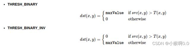
THRESH_BINARY表示大于thresh的取maxval,否则取0;THRESH_BINARY_INV表示大于thresh的取0,否则取maxvalue;THRESH_TRUNC表示大于thresh取threshold,否则不改变灰度值;THRESH_TOZERO表示大于thresh的不改变灰度值,否则取0;THRESH_TOZERO_INV表示大于thresh取0,窦泽不改变灰度值;THRESH_OTSU表示使用otsu自动计算阈值;THRESH_TRIANGLE表示使用Triangle自动计算阈值;
adaptiveThreshold
void adaptiveThreshold( InputArray src, OutputArray dst,
                       double maxValue, int adaptiveMethod,
                       int thresholdType, int blockSize, double C );
src表示需要进行二值化的图像;需要注意的是,该输入必须是8-bit单通道的图像;dst表示输出图像的二值图像;maxValue是一个非零值,用于对哪些满足条件的阈值进行赋值;adaptiveMethod表示选择哪一种自适应阈值算法;Opencv提供两种,ADAPTIVE_THRESH_MEAN_C与ADAPTIVE_THRESH_GAUSSIAN_C,下面会详细介绍;thresholdType表示二值化类型,OpenCV提供两种,THRESH_BINARY与THRESH_BINARY_INV,下面会详细介绍;blocksize表示参与计算的像素的领域范围,必须使用奇数;C可以为正数, 零或者负数;用于在计算过程中容忍程度;
thresholdType介绍
adaptiveMethod介绍
第一种ADAPTIVE_THRESH_MEAN_C,针对像素(x,y)的计算方式如下:
- T(x,y)结果是在(x,y)的邻域blockSize×blockSize范围内所有灰度值的均值减去C�;
第二种ADAPTIVE_THRESH_GAUSSIAN_C,针对像素(x,y)的计算方式如下:
- 首先,生成一个大小为blockSize×blockSize的高斯核,作为权重;
- 其次,利用高斯核与(x,y)邻域范围内灰度值,进行加权求和,再减去C,得到T(x,y);
高斯核:符合高斯分布,距离越近权重越大。
Canny
标准的边缘检测算法包括如下几步:
- 将图像转为灰度图像
- 通过高斯模糊卷积实现降噪
- 计算图像梯度的大小与角度
- 非最大信号压制
- 双阈值边缘连接
在图像利用Sobel算子(也是滤波函数)计算x, y两个方向的梯度:

其次,计算梯度的强度和方向:(根据X轴和Y轴方向的梯度可以计算图像中像素点的梯度幅值G与角度θ)

非最大抑制
理想情况下只有边缘像素的梯度是大于阈值T的,但实际情况下,局部也会出现多个高梯度阈值,所以要需要每个像素根据自身角度方向与两侧像素梯度值进行比较,如果当前像素点的梯度值小于两侧像素的梯度值,则将当前像素点的值设置为0;如果大于两侧像素的梯度值则保留。
双阈值连接
双阈值连接时保证边缘连续的关键步骤。一个高阈值H,一个低阈值L。
双阈值连接首先使用L对梯度图像进行处理,高于L保留,低于L丢弃,并将值设为零。然后使用H进行处理,高于H都视为边缘像素点。梯度值在[L,H]之间的:如果从低阈值像素点出发,最终可以通过相邻的像素点连接到高阈值像素点,而且整个连线上的像素点梯度值都大于L,则保留;否则设置为0。
轮廓发现与轮廓绘制
轮廓发现:
void findContours//提取轮廓,用于提取图像的轮廓
(
InputOutputArray image,//输入图像,必须是8位单通道图像,并且应该转化成二值的
OutputArrayOfArrays contours,//检测到的轮廓,每个轮廓被表示成一个point向量
OutputArray hierarchy,//可选的输出向量,包含图像的拓扑信息。其中元素的个数和检测到的轮廓的数量相等
int mode,//说明需要的轮廓类型和希望的返回值方式
int method,//轮廓近似方法
Point offset = Point()
)
轮廓绘制:
void drawContours//绘制轮廓,用于绘制找到的图像轮廓
(
 InputOutputArray image,//要绘制轮廓的图像
 InputArrayOfArrays contours,//所有输入的轮廓,每个轮廓被保存成一个point向量
 int contourIdx,//指定要绘制轮廓的编号,如果是负数,则绘制所有的轮廓
 const Scalar& color,//绘制轮廓所用的颜色
 int thickness = 1, //绘制轮廓的线的粗细,如果是负数,则轮廓内部被填充
 int lineType = 8, /绘制轮廓的线的连通性
 InputArray hierarchy = noArray(),//关于层级的可选参数,只有绘制部分轮廓时才会用到
 int maxLevel = INT_MAX,//绘制轮廓的最高级别,这个参数只有hierarchy有效的时候才有效
                                          //maxLevel=0,绘制与输入轮廓属于同一等级的所有轮廓即输入轮廓和与其相邻的轮廓
                                          //maxLevel=1, 绘制与输入轮廓同一等级的所有轮廓与其子节点。
                                          //maxLevel=2,绘制与输入轮廓同一等级的所有轮廓与其子节点以及子节点的子节点
 Point offset = Point()
)
代码示例:
void BinaryAnalysis::find_contours_demo(Mat &image) {
	Mat gray;
	cvtColor(image, gray, COLOR_BGR2GRAY);
	std::vector> contours;
	vector hierarchy;
	findContours(gray, contours, hierarchy, RETR_EXTERNAL, CHAIN_APPROX_SIMPLE, Point());
	Mat result = Mat::zeros(image.size(), image.type());
	drawContours(result, contours, -1, Scalar(0, 0, 255), 2, 8);
	imshow("轮廓发现", result);
}
轮廓测量
轮廓测量指对二值图像的每个轮廓的弧长和面积进行测量,根据轮廓的面积和弧长对大小不同的对象实现查找、过滤与处理的操作,以寻找感兴趣的RoI区域。
计算面积:
//计算面积
double cv::contourArea(
    InputArray contour
    bool oriented = false
)
//计算弧长、周长
double cv::arcLength(
    InputArray curve
    bool closed
    )
//计算轮廓外接矩形
Rect cv::boundingRect(
    InputArray array
)
//示例代码
void BinaryAnalysis::contours_analysis_demo(Mat &image) {
	// 二值化
	Mat gray, binary;
	cvtColor(image, gray, COLOR_BGR2GRAY);
	double t = threshold(gray, binary, 0, 255, THRESH_BINARY | THRESH_OTSU);

	// 轮廓发现
	std::vector> contours;
	vector hierarchy;
	findContours(binary, contours, hierarchy, RETR_EXTERNAL, CHAIN_APPROX_SIMPLE, Point());
	Mat result = Mat::zeros(image.size(), image.type());
	drawContours(result, contours, -1, Scalar(0, 0, 255), 2, 8);

	// 轮廓测量
	for (size_t t = 0; t < contours.size(); t++) {
		Rect box = boundingRect(contours[t]);

		double area = contourArea(contours[t]);
		double arc = arcLength(contours[t], true);
		putText(result, format("area:%.2f", area), box.tl(), FONT_HERSHEY_PLAIN, 1.0, Scalar(0, 255, 0), 1, 8);
		putText(result, format("arc:%.2f", arc), Point(box.x, box.y+14), FONT_HERSHEY_PLAIN, 1.0, Scalar(0, 255, 0), 1, 8);
	}
	imshow("轮廓测量", result);
}
轮廓拟合逼近
//拟合椭圆
RotatedRect cv::fitEllipse(
    InputArray
)
//拟合直线
void cv::fitLine(
    InputArray points
    OutputArray line
    int distType,
    double param,
    double reps,
    double aeps
)//distType表示拟合时使用的距离计算公式、、param表示对模型进行拟合距离计算的公式是否需要用到该参数。当distType参数为5,6,7时表示需要用到该参数,否则该参数不参与拟合距离计算、、reps与aeps表示对拟合结果的精度要求
//轮廓逼近
void cv::approxPolyDP(
    InputArray curve
    OutputArray approxCurve
    double epsilon
    bool closed
)
轮廓椭圆拟合与直线拟合示例代码:
//示例代码
void BinaryAnalysis::contours_fitness_demo(Mat &image) {
	// 二值化
	Mat edges;
	int t = 80;
	Canny(image, edges, t, t * 2, 3, false);
    //返回一个结构元素(卷积核),主要用于后续的膨胀腐蚀操作
	Mat k = getStructuringElement(MORPH_RECT, Size(3, 3), Point(-1, -1));
	//膨胀函数对于3*3的核,取最大的数放在中心位置
    dilate(edges, edges, k);

	// 轮廓发现
	std::vector> contours;
	vector hierarchy;
	findContours(edges, contours, hierarchy, RETR_EXTERNAL, CHAIN_APPROX_SIMPLE, Point());

	for (size_t t = 0; t < contours.size(); t++) {
		if (contours[t].size() < 5) {
			continue;
		}
		// 拟合椭圆
		// RotatedRect rrt = fitEllipse(contours[t]);
		// ellipse(image, rrt, Scalar(0, 0, 255), 2, 8);

		// 拟合直线
		Vec4f oneline;
		fitLine(contours[t], oneline, DIST_L1, 0, 0.01, 0.01);
		float vx = oneline[0];
		float vy = oneline[1];
		float x0 = oneline[2];
		float y0 = oneline[3];

		// 直线参数斜率k与截矩b
		float k = vy / vx;
		float b = y0 - k*x0;
		// 寻找轮廓极值点
		int minx = 0, miny = 10000;
		int maxx = 0, maxy = 0;
		for (int i = 0; i < contours[t].size(); i++) {
			Point pt = contours[t][i];
			if (miny > pt.y) {
				miny = pt.y;
			}
			if (maxy < pt.y) {
				maxy = pt.y;
			}
		}
		maxx = (maxy - b) / k;
		minx = (miny - b) / k;
		line(image, Point(maxx, maxy), Point(minx, miny), Scalar(0, 0, 255), 2, 8, 0);
	}
	imshow("轮廓拟合-直线拟合", image);
}
轮廓逼近示例代码:
void BinaryAnalysis::contours_apprv_demo(Mat &image) {
	Mat gray, binary;
	cvtColor(image, gray, COLOR_BGR2GRAY);
	double t = threshold(gray, binary, 0, 255, THRESH_BINARY | THRESH_OTSU);
	std::vector> contours;
	vector hierarchy;
	findContours(binary, contours, hierarchy, RETR_EXTERNAL, CHAIN_APPROX_SIMPLE, Point());
	for (size_t t = 0; t < contours.size(); t++) {
		std::vector pts;
		approxPolyDP(contours[t], pts, 10, true);
		for (int i = 0; i < pts.size(); i++) {
			circle(image, pts[i], 3, Scalar(0, 0, 255), 2, 8, 0);
		}
	}
	imshow("轮廓逼近", image);
}
轮廓分析
可以根据轮廓发现得到的每个对象轮廓的最大外接矩形活最小外接矩形计算其横纵比,周长,面积。
下面的示例代码使用了轮廓测量与分析的相关函数,完成了对每个对象轮廓的分析,得到了每个对象轮廓的属性输出。
void BinaryAnalysis::contours_attrs_demo(Mat &image) {
	// 二值化
	Mat edges;
	int t = 80;
	Canny(image, edges, t, t * 2, 3, false);

	Mat k = getStructuringElement(MORPH_RECT, Size(3, 3), Point(-1, -1));
	dilate(edges, edges, k);

	// 轮廓发现
	std::vector> contours;
	vector hierarchy;
	findContours(edges, contours, hierarchy, RETR_EXTERNAL, CHAIN_APPROX_SIMPLE, Point());
	Mat result = Mat::zeros(image.size(), image.type());
	drawContours(result, contours, -1, Scalar(0, 0, 255), 2, 8);
	imshow("轮廓发现", result);

	Mat mask = Mat::zeros(image.size(), CV_8UC1);
	for (size_t t = 0; t < contours.size(); t++) {
		Rect box = boundingRect(contours[t]);
		RotatedRect rrt = minAreaRect(contours[t]);
		std::vector hulls;
		convexHull(contours[t], hulls);
		double hull_area = contourArea(hulls);
		double box_area = box.width*box.height;
		double area = contourArea(contours[t]);
		// 计算横纵比
		double aspect_ratio = saturate_cast(rrt.size.width) / saturate_cast(rrt.size.height);
		// 计算延展度
		double extent = area / box_area;
		// 计算实密度
		double solidity = area / hull_area;
		// 生成mask与计算像素均值
		mask.setTo(Scalar(0));
		drawContours(mask, contours, t, Scalar(255), -1);
		Scalar bgra = mean(image, mask);
		putText(image, format("extent:%.2f", extent), box.tl(), FONT_HERSHEY_PLAIN, 1.0, Scalar(0, 0, 255), 1, 8);
		putText(image, format("solidity:%.2f", solidity), Point(box.x, box.y + 14), FONT_HERSHEY_PLAIN, 1.0, Scalar(0, 0, 255), 1, 8);
		putText(image, format("aspect_ratio:%.2f", aspect_ratio), Point(box.x, box.y + 28), FONT_HERSHEY_PLAIN, 1.0, Scalar(0, 0, 255), 1, 8);
		putText(image, format("mean:(%d,%d,%d)", (int)bgra[0], (int)bgra[1], (int)bgra[2]), Point(box.x, box.y + 42), FONT_HERSHEY_PLAIN, 1.0, Scalar(0, 0, 255), 1, 8);
	}
	imshow("轮廓分析", image);
}
直线检测圆检测
在二值图像分析中,直线检测和轮廓发现是经常遇到的处理要求。Opencv中的直线检测是基于霍夫变换完成的。
//标准霍夫直线检测
void cv::HoughLines(
    InputArray image
    OutputArray lines
    double rho    //距离步长d=1,指该直线到原点的距离,对于屏幕坐标,原点是左上角的点
    double theta    //角度步长
    int threshold    //
    double srn =0
    double stn=0
    double min_theta=0
    double max_theta=CV_PI
)
//概率霍夫直线检测
void cv::HoughLinesP(
    InputArray image
    OutputArray lines
    double rho
    double theta
    int threshold
    double minLineLength=0
    double maxLineGap=0
)
//霍夫圆检测
void cv::HoughCircle(
    InputArray image
    OutputArray circles//输出圆心与直径
    int method     //方法,当前只支持基于梯度的方法
    double dp    //关键参数,累加分辨率
    double minDist //两个圆之间的最小距离
    double param1=100 //边缘检测中的高梯度阈值
    double param2=100 //边缘检测中的低梯度阈值
    int minRadius=0 //最小圆半径
    int maxRadius=0 //最大圆半径
)
示例代码:
void BinaryAnalysis::hough_line_demo(Mat &image) {
	Mat edges;
	Canny(image, edges, 50, 200, 3);
	vector lines;
	HoughLines(edges, lines, 1, CV_PI / 180, 150, 0, 0);
	Mat result1, result2;
	cvtColor(edges, result1, COLOR_GRAY2BGR);
	result2 = result1.clone();
	for (size_t i = 0; i < lines.size(); i++)
	{
		float rho = lines[i][0], theta = lines[i][1];
		Point pt1, pt2;
		double a = cos(theta), b = sin(theta);
		double x0 = a*rho, y0 = b*rho;
		pt1.x = cvRound(x0 + 1000 * (-b));
		pt1.y = cvRound(y0 + 1000 * (a));
		pt2.x = cvRound(x0 - 1000 * (-b));
		pt2.y = cvRound(y0 - 1000 * (a));
		line(result1, pt1, pt2, Scalar(0, 0, 255), 3, LINE_AA);
	}
	imshow("标准霍夫直线检测", result1);

	// 概率霍夫直线检测
	vector linesP;
	HoughLinesP(edges, linesP, 1, CV_PI / 180, 50, 50, 10);
	for (size_t t = 0; t < linesP.size(); t++) {
		Point p1 = Point(linesP[t][0], linesP[t][1]);
		Point p2 = Point(linesP[t][2], linesP[t][3]);
		line(result2, p1, p2, Scalar(0, 0, 255), 2, 8, 0);
	}
	imshow("概率霍夫直线检测", result2);
}

void BinaryAnalysis::hough_circle_demo(Mat &image) {
	Mat gray;
	cvtColor(image, gray, COLOR_BGR2GRAY);
	GaussianBlur(gray, gray, Size(5, 5), 0, 0);
	std::vector circles;
	HoughCircles(gray, circles, HOUGH_GRADIENT_ALT, 2, 10, 100, 50, 20, 40);
	for (size_t t = 0; t < circles.size(); t++) {
		Vec3f c = circles[t];
		Point center = Point(c[0], c[1]);
		int radius = c[2];
		circle(image, center, radius, Scalar(255, 0, 255), 2, 8, 0);
		circle(image, center, 3, Scalar(255, 0, 0), 3, 8, 0);
	}
	imshow("霍夫圆检测", image);
}
最大内接圆与最小外接圆
opencv未提供API函数来寻找最大内接圆,但是可以通过点多边形测试函数巧妙地获取轮廓最大内接圆地半径,从而找到最大内接圆。
//最小外接圆
void cv::minEnclosingCircle(
    InputArray pooints
    Point2f & center
    float & radius
)
//点多边形测试函数
double cv::pointPolygonTest(
    InputArray contour
    Point2f pt
    bool measureDist //是否测量距离,当measureDist设置为true时,返回的是该点到轮廓的真是距离。设置为false时,返回的是+1、0、-1
)
//示例代码
void BinaryAnalysis::inner_extenerl_circle_demo(Mat &image) {
	Mat gray;
	cvtColor(image, gray, COLOR_BGR2GRAY);
	std::vector> contours;
	vector hierarchy;
	findContours(gray, contours, hierarchy, RETR_EXTERNAL, CHAIN_APPROX_SIMPLE, Point());
	for (size_t t = 0; t < contours.size(); t++) {
		// 最小外接圆
		Point2f pt;
		float radius;
		minEnclosingCircle(contours[t], pt, radius);
		circle(image, pt, radius, Scalar(255, 0, 0), 2, 8, 0);

		// 点多边形测试
		Mat raw_dist(image.size(), CV_32F);
		for (int i = 0; i < image.rows; i++)
		{
			for (int j = 0; j < image.cols; j++)
			{
				raw_dist.at(i, j) = (float)pointPolygonTest(contours[t], Point2f((float)j, (float)i), true);
			}
		}

		// 获取最大内接圆半径
		double minVal, maxVal;
		Point maxDistPt; // inscribed circle center
		minMaxLoc(raw_dist, &minVal, &maxVal, NULL, &maxDistPt);
		minVal = abs(minVal);
		maxVal = abs(maxVal);
		circle(image, maxDistPt, maxVal, Scalar(0, 0, 255), 2, 8, 0);
	}
	imshow("最大内接圆与最小外接圆演示", image);
}
轮廓匹配
二值图像轮廓发现可以得到每个圆形的轮廓,然后计算轮廓几何矩,再根据几何矩计算图像的中心位置。根据中心位置计算中心距,然后根据中心距计算中心归一化距。再根据归一化距计算胡距,最后比较轮廓胡距之间的相似性,从而实现轮廓匹配。
//几何矩、中心距、中心归一化距可通过moments函数一次就计算出来
Moments cv::moments(
    InoutArray array
    bool binaryImage=false //是否为二值图像
)

void cv::HuMoments(
    const Moments & moments
    double hu[7] //胡距的7个值
)
//将胡距作为输入,对轮廓进行匹配。胡距具有缩放不变性与旋转不变性,所以进行轮廓外形匹配时,可以匹配到旋转与分辨率不一样的同一个轮廓。
//轮廓匹配函数
double cv::matchShapes(
    InputArray contour1
    InputArray contour2
    int method //比较方法
    double parameter //opencv3.x以后不需要
)
//示例代码
void BinaryAnalysis::contour_match_demo(Mat &image) {
	Mat src = imread("D:/images/abc.png");
	imshow("input", src);
	Mat src2 = imread("D:/images/a5.png");
	namedWindow("input2", WINDOW_FREERATIO);
	imshow("input2", src2);

	// 轮廓提取
	vector> contours1;
	vector> contours2;
	contours_info(src, contours1);
	contours_info(src2, contours2);
	// hu矩计算
	Moments mm2 = moments(contours2[0]);
	Mat hu2;
	HuMoments(mm2, hu2);
	// 轮廓匹配
	for (size_t t = 0; t < contours1.size(); t++) {
		Moments mm = moments(contours1[t]);
		Mat hum;
		HuMoments(mm, hum);
		double dist = matchShapes(hum, hu2, CONTOURS_MATCH_I1, 0);
		printf("contour match distance : %.2f\n", dist);
		if (dist < 1) {
			printf("draw it \n");
			Rect box = boundingRect(contours1[t]);
			rectangle(src, box, Scalar(0, 0, 255), 2, 8, 0);
		}
	}
	imshow("match result", src);
}
最大轮廓与关键点编码
根据二值图像实现轮廓发现,分析每个轮廓并根据面积找到最大轮廓,对最大轮廓使用轮廓逼近,从而得到轮廓编码点。最后绘制编码点信息并显示。
void BinaryAnalysis::max_contour_demo(Mat &image) {
	// 二值图像
	Mat mask;
	inRange(image, Scalar(0, 0, 0), Scalar(110, 110, 110), mask);
	bitwise_not(mask, mask);

	// 轮廓发现
	vector> contours;
	vector hierarchy;
	findContours(mask, contours, hierarchy, RETR_EXTERNAL, CHAIN_APPROX_SIMPLE);
	int height = image.rows;
	int width = image.cols;
	int index = -1;
	int max = 0;

	// 最大轮廓寻找
	for (size_t t = 0; t < contours.size(); t++) {
		double area = contourArea(contours[t]);
		if (area > max) {
			max = area;
			index = t;
		}
	}
	Mat result = Mat::zeros(image.size(), image.type());
	Mat pts;
	drawContours(result, contours, index, Scalar(0, 0, 255), 1, 8);

	// 关键点编码提取与绘制
	approxPolyDP(contours[index], pts, 4, true);
	for (int i = 0; i < pts.rows; i++) {
		Vec2i pt = pts.at(i, 0);
		circle(result, Point(pt[0], pt[1]), 2, Scalar(0, 255, 0), 2, 8, 0);
		circle(result, Point(pt[0], pt[1]), 2, Scalar(0, 255, 0), 2, 8, 0);
	}
	imshow("最大轮廓与关键点编码", result);
}
凸包检测
//轮廓提取凸包
void cv::convexHull(
    InputArray points
    OutputArray hull
    bool clockwise = false
    bool returnPoints =true//是否返回点集
)
//判断轮廓是否为凸包
bool cv::isContourConvex(
    InputArray contour
)

//示例代码
void BinaryAnalysis::convex_demo(Mat &image) {
	vector> contours;
	contours_info(image, contours);
	for (size_t t = 0; t < contours.size(); t++) {
		vector hull;
		convexHull(contours[t], hull);
		bool isHull = isContourConvex(contours[t]);
		printf("test convex of the contours %s \n", isHull ? "Y" : "N");
		int len = hull.size();
		for (int i = 0; i < hull.size(); i++) {
			circle(image, hull[i], 4, Scalar(255, 0, 0), 2, 8, 0);
			line(image, hull[i%len], hull[(i + 1) % len], Scalar(0, 0, 255), 2, 8, 0);
		}
	}
	imshow("凸包检测", image);
}