DS Wannabe之5-AM Project: DS 30day int prep day2

Q1. What is Logistic Regression?

The logistic regression technique involves the dependent variable, which can be represented in the binary (0 or 1, true or false, yes or no) values, which means that the outcome could only be in either one form of two. For example, it can be utilized when we need to find the probability of a successful or fail event.

If ‘Z’ goes to infinity, Y(predicted) will become 1, and if ‘Z’ goes to negative infinity, Y(predicted) will become 0.
The output from the hypothesis is the estimated probability. This is used to infer how confident can predicted value be actual value when given an input X.

Q2. Difference between logistic and linear regression?

Linear and Logistic regression are the most basic form of regression which are commonly used. The essential difference between these two is that Logistic regression is used when the dependent variable is binary. In contrast, Linear regression is used when the dependent variable is continuous, and the nature of the regression line is linear.

Key Differences between Linear and Logistic Regression

Linear regression models data using continuous numeric value. As against, logistic regression models the data in the binary values.
Linear regression requires to establish the linear relationship among dependent and independent variables, whereas it is not necessary for logistic regression.

In linear regression, the independent variable can be correlated with each other. On the contrary, in the logistic regression, the variable must not be correlated with each other.

Q3. Why we can’t do a classification problem using Regression?

Linear regression is unbounded.

Q4. What is Decision Tree?

A decision tree is a type of supervised learning algorithm that can be used in classification as well as regressor problems.

Decision tree is a tree-based method that goes from observations about an object (represented in the branches) to conclusions about its target value (represented in the leaves). At its core, decision trees are nest if-else conditions.

In classification trees, the target value is discrete and each leaf represents a class. In regression trees, the target value is continuous and each leaf represents the mean of the target values of all objects that end up with that leaf.

Decision trees are easy to interpret and can be used to visualize decisions. However, they are overfit to the data they are trained on -- small changes to the training set can result in significantly different tree structures, which lead to significantly different outputs.

The input to a decision tree can be both continuous as well as categorical. The decision tree works on an if-then statement. Decision tree tries to solve a problem by using tree representation (Node and Leaf)

Assumptions while creating a decision tree:

1) Initially all the training set is considered as a root

2) Feature values are preferred to be categorical, if continuous then they are discretized

3) Records are distributed recursively on the basis of attribute values

4) Which attributes are considered to be in root node or internal node is done by using a statistical approach.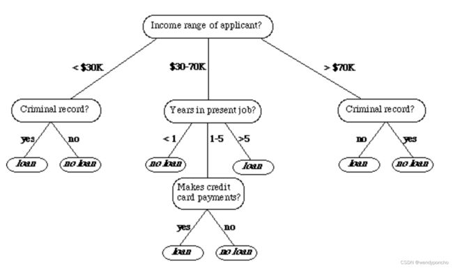

创建决策树时的假设包括：

1. 最初，所有的训练集被视为根节点。
2. 特征值最好是分类的，如果是连续的，则需要离散化。
3. 根据属性值递归地分配记录。
4. 通过使用统计方法来确定哪些属性应被视为根节点或内部节点。

Q5. Entropy, Information Gain, Gini Index, Reducing Impurity?

在构建决策树时，选择最佳分裂属性的关键指标包括熵、信息增益、基尼指数和纯度降低。这些概念帮助我们评估每个属性对于数据集划分的有效性，从而构建一个高效的决策树模型。

熵 (Entropy)

熵是衡量数据集中不确定性或混乱程度的指标。在决策树中，熵用于评估数据集的纯度。

熵是从0到1变化的，当所有数据都属于单一类别时熵为0，当类别分布完全平均时熵为1。这样，熵可以用来衡量数据集中的不纯度。

选择哪个属性进行分裂的步骤如下：

1. 计算整个数据集的熵。
2. 对于每个属性： 2.1 计算所有分类值的熵。 2.2 计算该属性的平均信息熵。 2.3 计算当前属性的信息增益。
3. 选择信息增益最高的属性。
4. 重复上述过程直到得到所需的树结构。

当熵为零时确定为叶节点。

信息增益 = 1 - ∑ (Sb/S) * 熵(Sb)，其中Sb是子集，S是整个数据集。这个过程有助于确定哪个属性在分裂时能最大程度地减少数据集的不纯度，进而提高决策树模型的效率和准确度。通过重复这一过程，我们可以逐步构建出决策树，直到每个叶节点的熵都为零，即每个叶节点都纯粹地包含同一类别的数据。

其中，pi​ 是选择第i类的概率。

Entropy varies from 0 to 1. 0 if all the data belong to a single class and 1 if the class distribution is equal. In this way, entropy will give a measure of impurity in the dataset.
Steps to decide which attribute to split:

1. Computetheentropyforthedataset

2. Foreveryattribute:

2.1 Calculate entropy for all categorical values.

  2.2 Take average information entropy for the attribute.

  2.3 Calculate gain for the current attribute.
3. Picktheattributewiththehighestinformationgain.

4. Repeat until we get the desired tree.

A leaf node is decided when entropy is zero

Information Gain = 1 - ∑ (Sb/S)*Entropy (Sb) Sb - Subset, S - entire data

信息增益 (Information Gain)

信息增益是基于熵的概念，它衡量通过对数据集进行分裂后熵的减少（即纯度的增加）。在决策树中，我们倾向于选择那些能带来最大信息增益的属性作为分裂属性。

信息增益公式

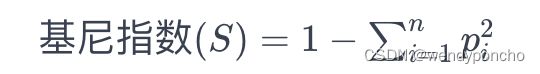
基尼指数 (Gini Index)

基尼指数是另一种衡量数据集纯度的方法，常用于CART（分类和回归树）算法。基尼指数衡量的是从数据集中随机选取两个项，它们属于不同类别的概率。基尼指数越小，数据集的纯度越高。

基尼指数公式

CART算法（Classification and Regression Trees，分类和回归树）是一种决策树学习算法，它可以用于分类问题也可以用于回归问题。在CART算法中，我们使用基尼指数（Gini Index）作为评估数据集分裂的指标，基尼指数被用作成本函数来评估数据集的分裂。

计算分裂的基尼指数的步骤如下：

1. 计算子节点的基尼指数：通过使用公式，即成功和失败的概率的平方和（p2+q2），来计算子节点的基尼指数。这里的p表示成功（或某一类别）的概率，而q=1−p则表示失败（或其他类别）的概率。

2. 计算分裂的基尼指数：通过计算该分裂中每个节点的加权基尼得分来计算分裂的基尼指数。加权基尼得分是指将每个子节点的基尼指数乘以该节点在分裂中所占的比重（即该节点样本数占总样本数的比例。

在这个例子中，我们使用基尼指数来评估基于不同属性（如性别和班级）进行分裂的决策树节点的纯度。

当我们根据性别属性进行分裂时：

• 对于女性子节点，基尼指数计算为 0.680.68，计算方式为 (0.2)∗(0.2)+(0.8)∗(0.8)(0.2)∗(0.2)+(0.8)∗(0.8)，其中 0.20.2 和 0.80.8 分别是某类别（比如成功或者某个特定分类）的概率及其补概率。
• 对于男性子节点，基尼指数计算为 0.550.55，计算方式为 (0.65)∗(0.65)+(0.35)∗(0.35)(0.65)∗(0.65)+(0.35)∗(0.35)。
• 性别分裂的加权基尼指数为 0.590.59，计算方式为 (10/30)∗0.68+(20/30)∗0.55(10/30)∗0.68+(20/30)∗0.55，其中 10/3010/30 和 20/3020/30 分别是女性和男性子节点在所有数据中的比重。

当我们根据班级属性进行分裂时：

• 对于班级IX子节点，基尼指数为 0.510.51，计算方式与上述相同。
• 对于班级X子节点，基尼指数也为 0.510.51。
• 班级分裂的加权基尼指数为 0.510.51，计算方式为 (14/30)∗0.51+(16/30)∗0.51(14/30)∗0.51+(16/30)∗0.51，其中 14/3014/30 和 16/3016/30 分别是班级IX和X子节点在所有数据中的比重。

在这两个分裂选项中，性别分裂的加权基尼指数更高（0.59），而班级分裂的加权基尼指数较低（0.51）。在CART算法中，我们倾向于选择那些能使基尼指数最小化的分裂属性，因为较低的基尼指数表示更高的数据纯度。因此，在这个例子中，我们会选择基于班级属性进行分裂，因为它提供了较低的加权基尼指数，从而意味着在这次分裂后数据的纯度更高。

基尼指数越小，表示数据集的纯度越高，即数据集中包含的类别越单一。因此，在CART算法中，我们会选择那些能够产生最小基尼指数的属性来进行分裂，以此构建决策树，直到达到某个停止条件，如节点中的样本数量低于某个阈值，或者所有节点的基尼指数都已经很低了。这样构建出来的决策树能够有效地对数据进行分类或回归预测。

减少不纯度 (Reducing Impurity)

在构建决策树时，目标是选择最佳的分裂属性，以最大化不纯度的减少。通过比较不同分裂方案的熵、信息增益或基尼指数，可以确定哪种分裂最能提高节点的纯度。减少不纯度有助于构建更准确、更简洁的决策树模型，减少过拟合的风险，并提高模型的泛化能力。

Q6. How to control leaf height and Pruning?

控制叶节点大小和剪枝是决策树模型优化的重要方面，有助于防止过拟合并提高模型的泛化能力

To control the leaf size, we can set the parameters: 

1. Maximum depth: 最大深度
Maximum tree depth is a limit to stop the further splitting of nodes when the specified tree depth has been reached during the building of the initial decision tree.
NEVER use maximum depth to limit the further splitting of nodes. In other words: use the largest possible value.

2. Minimum split size: 最小分裂大小
Minimum split size is a limit to stop the further splitting of nodes when the number of observations in the node is lower than the minimum split size.
This is a good way to limit the growth of the tree. When a leaf contains too few observations, further splitting will result in overfitting (modeling of noise in the data).

3. Minimum leaf size 最小叶节点大小
Minimum leaf size is a limit to split a node when the number of observations in one of the child nodes is lower than the minimum leaf size.
Pruning is mostly done to reduce the chances of overfitting the tree to the training data and reduce the overall complexity of the tree.

剪枝

剪枝主要用于减少树对训练数据过拟合的风险，并降低树的整体复杂度。剪枝有两种类型：预剪枝和后剪枝。

预剪枝（Pre-pruning）：也称为提前停止准则。顾名思义，这些准则作为在构建模型时设置的参数值。当决策树在生长过程中遇到任何这些预剪枝准则，或者发现纯净的类别时，就会停止生长。

1. Pre-pruning is also known as the early stopping criteria.As the name suggests,the criteria are set as parameter values while building the model. The tree stops growing when it meets any of these pre-pruning criteria, or it discovers the pure classes.

2. In Post-pruning,the idea is to allow the decision tree to growfully and observe the CP value. Next, we prune/cut the tree with the optimal CP(Complexity Parameter) value as the parameter. The CP (complexity parameter) is used to control tree growth. If the cost of adding a variable is higher, then the value of CP, tree growth stops.

在后剪枝（Post-pruning）中，策略是允许决策树完全生长，然后观察复杂度参数（CP，Complexity Parameter）的值。接下来，我们以最优的CP值作为参数来剪枝/裁剪树。CP用于控制树的生长，如果添加一个变量的成本高于CP的值，树的生长就会停止。

后剪枝的过程包括以下步骤：

1. 完全生长：首先允许决策树完全生长，直到每个叶节点都是纯净的，或者直到达到其他预先定义的停止条件。

2. 计算CP值：对于树的每个节点，计算如果从该节点开始剪枝将导致的性能损失与树复杂度减少的比率，这个比率就是CP值。性能通常是通过验证集上的误差来衡量的，而复杂度则与树中的节点数有关。

3. 选择最优CP：通过观察不同CP值对模型性能的影响，选择一个最优的CP值。最优的CP值是指在不显著增加验证集上的误差的情况下能最大程度减少树的复杂度的CP值。

4. 剪枝：使用选定的最优CP值对树进行剪枝。具体来说，从树的底部开始，如果删除某个节点（及其所有子节点）导致的性能损失小于或等于CP值所允许的损失，则执行剪枝操作。

后剪枝是一种有效的剪枝技术，因为它在剪枝决策时考虑了树的整体性能，通常能产生比预剪枝更准确的模型。通过这种方式，可以在保持模型性能的同时减少模型的复杂度，避免过拟合，并提高模型在未见数据上的泛化能力。

Q7. How to handle a decision tree for numerical and categorical data?

Decision trees can handle both categorical and numerical variables at the same time as features. There is not any problem in doing that.

决策树能够同时处理分类数据和数值数据作为特征，这在决策树的构建中并不构成问题。

决策树的每一次分裂都是基于某个特征来进行的：

1. 如果特征是分类的，分裂可以根据元素是否属于特定类别来进行。例如，如果一个特征是颜色，且其值可以是“红色”、“蓝色”或“绿色”，那么决策树可能会在“颜色=红色”处进行一次分裂，将数据分为“红色”和“非红色”两部分。

2. 如果特征是连续的，分裂则是基于是否超过某个阈值来进行的。例如，如果一个特征是年龄，决策树可能会在“年龄>30”处进行一次分裂，将数据分为年龄大于30和小于等于30的两部分。

在每一次分裂时，决策树会选择当前最佳的变量，这一选择是根据分裂后的不纯度衡量标准来进行的。使用的变量是分类的还是连续的对于决策树来说并不重要，因为决策树通过创建以阈值为界的二进制区域来将连续变量进行“分类”。

最后，将分类变量转换为连续变量是一种好的做法。这可以通过标签编码（Label Encoding）或独热编码（One-Hot Encoding）来实现。标签编码将每个类别赋予一个唯一的整数，而独热编码则为每个类别创建一个新的二进制列，对应类别的列值为1，其他为0。这两种编码方式能够帮助决策树更好地理解和分割数据，尤其是在处理具有多个类别的分类特征时。

Q8. What is the Random Forest Algorithm?

随机森林是一种集成学习算法，遵循装袋技术（bagging）。基于对决策树应用装袋（bagging）方法的算法，但它有一个重要的扩展：除了对记录进行抽样外，该算法还对变量进行抽样。在传统的决策树中，为了决定如何创建分区A的一个子分区，算法通过最小化诸如基尼不纯度（Gini impurity）这样的标准来选择变量和分割点。而在随机森林中，算法在每个阶段限制变量的选择为随机选定的变量子集。

随机森林模型的步骤如下：

1. 创建随机子集：从原始数据集中创建随机子集（通过自助采样法，即有放回的抽样）。
2. 节点的随机特征选择：在决策树的每个节点，仅考虑一组随机选定的特征来决定最佳的分裂点。
3. 拟合决策树模型：在每个子集上拟合一个决策树模型。
4. 最终预测的计算：通过汇总所有决策树的预测结果来计算最终预测，通常是通过取平均值。

总而言之，随机森林通过随机选择数据点和特征，并构建多棵树（即“森林”）来进行预测。

随机森林也用于特征重要性选择。通过使用属性（.feature_importances_），可以评估各个特征对模型预测能力的贡献大小，这对于理解数据中哪些特征是决定预测结果的关键因素非常有帮助。

与基本的树算法相比，随机森林算法增加了两个更多的步骤：之前讨论的装袋和在每个分裂点对变量进行自助采样（bootstrap sampling）：

1. 从记录中取一个带替换的自助子样本。
2. 对于第一个分裂点，随机无替换地抽样p个变量，其中p < P，P是预测变量的数量。
3. 对于每个抽样的变量：
   • 对于变量的每个值：
     • 将分区A中的记录分割为Xj(k) < sj(k)的一部分，以及剩余记录为另一部分。
     • 测量A的每个子分区内的类别同质性。
     • 选择产生最大类内同质性的值。
   • 选择产生最大类内同质性的变量和分割值。
4. 进行下一个分裂并重复之前的步骤，从第2步开始。
5. 继续进行更多的分裂，直到树完全生长。
6. 返回第1步，取另一个自助子样本，并重新开始这个过程。

每个步骤中应该抽样多少个变量？一个经验法则是选择 P​，其中P是预测变量的数量。randomForest 包在R中实现了随机森林算法。以下是将这个包应用于贷款数据的示例（参见“K-最近邻”了解数据的描述）：

predictors = ['borrower_score', 'payment_inc_ratio']
outcome = 'outcome'

X = loan3000[predictors]
y = loan3000[outcome]

rf = RandomForestClassifier(n_estimators=500, random_state=1, oob_score=True)
rf.fit(X, y)

随机森林通过这种方式结合了多个决策树的预测结果，通过对这些结果进行汇总（例如，通过投票或平均）来提高整体模型的准确性和稳定性。通过在每个分裂点随机选择变量，随机森林还增加了模型的多样性，这有助于降低过拟合的风险，提高模型在未见数据上的泛化能力。

Some Important Parameters:-

1. n_estimators:- It defines the number of decision trees to be created in a random forest.

2. criterion:- "Gini" or "Entropy."

3. min_samples_split:- Used to define the minimum number of samples required in a leaf

   node before a split is attempted

4. max_features: -It defines the maximum number of features allowed for the split in each

   decision tree.

5. n_jobs:- The number of jobs to run in parallel for both fit and predict. Always keep (-1) to

   use all the cores for parallel processing.

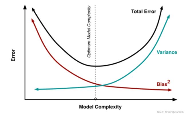
Q9. What is Variance and Bias tradeoff?

在预测模型中，预测误差由两种不同的误差组成：偏差（Bias）和方差（Variance）。理解偏差和方差之间的权衡对于最小化预测中的偏差和方差，并避免模型的过拟合和欠拟合非常重要。

偏差（Bias）

偏差是模型的预期或平均预测值与我们试图预测的正确值之间的差异。如果我们尝试通过收集不同的数据集构建不止一个模型，并在之后评估预测，我们可能会得到所有模型的不同预测结果。因此，偏差是衡量这些模型预测与正确预测有多远的一种方式。偏差往往导致在训练数据和测试数据上都有高误差。

高偏差通常是由于模型过于简单（欠拟合），没有捕捉到数据的基本趋势而造成的。在这种情况下，模型对训练数据和未见数据都不能进行准确的预测。

方差（Variance）

方差是指给定数据点的模型预测的可变性。我们可以多次构建模型，所以方差就是对于给定点的预测在不同模型实现之间变化的程度。高方差通常是由于模型过于复杂（过拟合），捕捉到了数据中的随机噪声而不仅仅是底层数据分布的特征。

当方差很高时，模型可能在训练数据上表现良好，但在新的、未见过的数据上表现不佳，因为它对训练数据中的随机波动做出了过度的反应。

偏差-方差权衡（Bias-Variance Tradeoff）

在模型的预测中，通常需要在偏差和方差之间找到一个平衡点。如果模型太简单，它可能具有高偏差和低方差；如果模型太复杂，它可能具有低偏差和高方差。理想的模型是在保持偏差和方差都相对较低的情况下做出准确的预测。

达到这种平衡通常涉及到模型选择、正则化技术（如L1、L2正则化）以及集成学习方法（如随机森林、梯度提升树等），这些方法旨在综合多个模型来提高预测的稳定性和准确性。

For example: Voting Republican - 13 Voting Democratic - 16 Non-Respondent - 21 Total - 50 The probability of voting Republican is 13/(13+16), or 44.8%. We put out our press release that the Democrats are going to win by over 10 points; but, when the election comes around, it turns out they lose by 10 points. That certainly reflects poorly on us.

Where did we go wrong in our model?

偏差的场景

• 使用电话簿选择参与者：这是偏差的一个来源。通过只调查电话簿中的某些人群，会以一种如果重复整个模型构建过程将保持一致的方式歪曲结果。这意味着如果你再次进行这样的调查，虽然结果可能会一致，但这种一致性是建立在对特定人群的有偏选择上的，这并不代表整个选民的真实意愿。
• 不跟进回应者：这也是偏差的一个来源。不跟进可能未能参与调查的人，会导致你获取的回应混合体系的一致性变化。这些偏差的来源使得你的预测系统性地偏离了真实值。

方差的场景

• 样本量小：这是方差的一个来源。如果增加样本量，每次重复调查和预测时得到的结果将更为一致。尽管由于存在较大的偏差源导致结果可能仍然高度不准确，但预测的方差将减少。

在这个例子中，主要问题似乎是由偏差引起的，特别是由于使用了可能不代表整个选民人群的抽样方法（如使用电话簿选择参与者），以及未能跟进所有潜在的回应者。这些偏差使得预测倾向于某一方，而不是准确反映整个选民的真实意愿。

为了改进模型并减少这种偏差，可以采取以下措施：

• 扩大和多样化样本：确保样本代表了整个选民人群的广泛特征，包括不同的社会经济背景、地理位置和其他相关因素。
• 改进抽样方法：使用更加随机和全面的抽样方法，而不是依赖于可能具有偏差的数据源（如电话簿）。
• 增加样本量：通过增加样本量来减少结果的方差，使得预测更加稳定和一致。

通过这些改进，可以提高模型的准确性和可靠性，从而避免类似的错误预测。

Q10. What are Ensemble Methods?

1. Bagging（自举聚合）

Bagging，全称为Bootstrap Aggregation，旨在通过减少决策树的方差来提高模型的稳定性和准确性。Bagging的过程如下：

• 从原始训练数据集中随机有放回地抽取多个子样本。
• 使用每个子样本独立训练一个决策树模型。
• 对于分类问题，使用投票机制来确定最终预测；对于回归问题，计算所有决策树预测的平均值。

Bagging is like the basic algorithm for ensembles, except that, instead of fitting the various models to the same data, each new model is fitted to a bootstrap resample. Here is the algorithm presented more formally:

1. Initialize M, the number of models to be fit, and n, the number of records to choose (n < N). Set the iteration m=1.

2. Take a bootstrap resample (i.e., with replacement) of n records from the training data to form a subsample Ym and m (the bag).

3. Train a model using Ym and m to create a set of decision rules f^m().

4. Increment the model counter m=m+1. If m <= M, go to step 2.

In the case where f^M predicts the probability Y=1, the bagged estimate is given by:

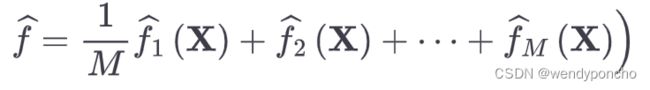
Bagging的一个典型例子是随机森林算法，其中多个决策树的预测结果被综合起来，以获得更稳定和准确的预测。

2. Boosting

Boosting方法通过顺序地训练一系列模型，每个模型都尝试修正前一个模型的错误。Boosting的关键步骤包括：

• 首先训练一个基本模型（如决策树）。
• 基于当前组合模型的错误率来调整数据的权重，使得之前模型预测错误的数据在后续模型中获得更多的关注。
• 添加新的模型，专注于更难预测的数据点。
• 这个过程重复进行，直到达到预定的模型数量，或模型性能不再显著提升。

在线性回归模型中，确实常常会检查残差，以判断模型的拟合情况是否可以改进。这种方法旨在识别数据中可能存在的非线性关系，从而优化模型的性能。Boosting方法将这一概念推向了极致，它通过拟合一系列模型来实现，其中每个后续模型都致力于最小化前一个模型的误差。Boosting方法的例子包括AdaBoost（自适应增强）和Gradient Boosting，它们都是通过增加后续模型对前一模型误差的关注来逐步提高模型的准确性。

总的来说，集成方法通过组合多个模型来提高预测的稳定性和准确性，有效地平衡了偏差和方差，从而提高了模型在未见数据上的泛化能力。

Boosting的变体

• Adaboost（自适应增强）：是Boosting方法的早期形式之一，通过增加之前被模型错误预测的观测值的权重，使得后续的模型更加关注这些难以预测的观测值。

• 梯度增强（Gradient Boosting）：通过使用损失函数的梯度来指导模型的改进。在每一步，梯度增强会添加一个新的模型，这个模型是在损失函数的梯度方向上对误差进行拟合，从而逐步减少整体误差。

• 随机梯度增强（Stochastic Gradient Boosting）：是梯度增强的一个变体，它通过在每一步随机选择样本和特征来增加随机性，从而提高模型的鲁棒性和减少过拟合的风险。这种方法是最通用和广泛使用的Boosting方法。

If these two methods were cars, bagging could be considered a Honda Accord (reliable and steady), whereas boosting could be considered a Porsche (powerful but requires more care).

Bagging（自举聚合）：本田雅阁（Honda Accord）

• 可靠性：正如本田雅阁以其可靠性和稳定性而闻名，Bagging通过构建多个独立的模型并对它们的预测进行平均或投票，提高了整体模型的稳定性和准确性。这种方法通过减少方差，使得最终的模型对训练数据中的随机波动不太敏感。
• 稳定性：Bagging不会过分关注任何特定的数据点，从而避免了过拟合的风险。这种稳定性使得Bagging类似于一辆性能可靠的本田雅阁，能够稳定地完成其任务，即使在不同的道路条件下。

Boosting：保时捷（Porsche）

• 强大：Boosting是一种将多个模型顺序地结合起来，每个模型都试图纠正前一个模型的错误的方法。这种方法可以显著提高模型的性能，类似于保时捷以其强大的性能而著称。
• 需要更多关注：Boosting方法对参数的选择和模型的设置更为敏感，可能需要更多的调整和细心的维护来避免过拟合。就像保时捷这样的高性能车辆可能需要更多的关注和维护一样，Boosting也需要更加小心地处理以确保最佳性能。

通过这种比喻，我们可以更直观地理解Bagging和Boosting在集成学习方法中的角色和特性。Bagging提供了稳定可靠的改进，而Boosting则提供了强大但需要精细调整的性能提升。选择哪种方法取决于特定问题的需求、数据的特性以及对模型复杂性和可解释性的偏好。

Q11. What is SVM Classification?

SVM or Large margin classifier is a supervised learning algorithm that uses a powerful technique called SVM for classification.

支持向量机（Support Vector Machine，简称SVM）是一种强大的监督学习算法，用于分类和回归任务。在分类问题中，SVM的目标是找到一个超平面（在二维空间中是一条直线，在更高维空间中是一个平面或超平面），这个超平面能够最好地分隔不同类别的数据点。

SVM分类的关键概念包括：

1. 最大边距

SVM试图找到一个超平面，不仅仅是能够分隔两个类别，而且在分隔两个类别时保持最大的边距（margin）。边距是指从超平面到最近的数据点（这些点被称为支持向量）的最短距离。最大化边距的想法旨在提高模型的泛化能力，因为它为数据的未见变化提供了更大的容错空间。

2. 支持向量

支持向量是距离分隔超平面最近的那些数据点。这些点是最难分隔的，因此直接决定了最终超平面的位置和方向。SVM模型的构建实际上只依赖于这些支持向量，而不是全部数据点，这使得模型不仅高效而且具有很好的鲁棒性。

3. 核技巧（Kernel Trick）

在实际应用中，很多数据集不是线性可分的，这意味着不能通过一个简单的直线或平面来分隔不同的类别。SVM通过引入核技巧来解决这个问题。核技巧通过将数据映射到更高维的空间来使原本线性不可分的数据变得可分。常用的核函数包括线性核、多项式核、径向基函数（RBF）核等。

4. 软间隔和正则化

在现实世界的数据中，往往存在噪声和异常点，这些点可能会违反最大边距准则。为了使SVM能够更好地处理这种情况，引入了软间隔的概念，允许某些数据点违反边距准则。这是通过引入松弛变量（slack variables）和正则化参数来实现的，正则化参数控制了对违反边距的容忍度与保持边距大小之间的权衡。

SVM因其优异的性能和强大的理论基础，在许多领域都得到了广泛应用，包括图像识别、生物信息学、文本分类等。

We have two types of SVM classifiers:

1) Linear SVM: In Linear SVM, the data points are expected to be separated by some apparent gap. Therefore, the SVM algorithm predicts a straight hyperplane dividing the two classes. The hyperplane is also called as maximum margin hyperplane

2) Non-Linear SVM: It is possible that our data points are not linearly separable in a p- dimensional space, but can be linearly separable in a higher dimension. Kernel tricks make it possible to draw nonlinear hyperplanes. Some standard kernels are a) Polynomial Kernel b) RBF kernel(mostly used).

Advantages of SVM classifier:
1) SVMs are effective when the number of features is quite large.
2) It works effectively even if the number of features is greater than the number of samples.
3) Non-Linear data can also be classified using customized hyperplanes built by using kernel trick. 4) It is a robust model to solve prediction problems since it maximizes margin.

Disadvantages of SVM classifier:

1) The biggest limitation of the Support Vector Machine is the choice of the kernel. The wrong choice of the kernel can lead to an increase in error percentage.
2) With a greater number of samples, it starts giving poor performances.
3) SVMs have good generalization performance, but they can be extremely slow in the test phase. 4) SVMs have high algorithmic complexity and extensive memory requirements due to the use of quadratic programming.

Q12. What is Naive Bayes Classification and Gaussian Naive Bayes?

Bayes’ Theorem finds the probability of an event occurring given the probability of another event that has already occurred. Bayes’ theorem is stated mathematically as the following equation:

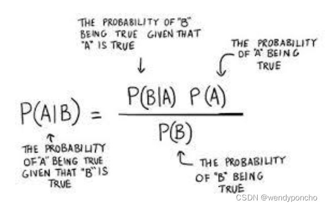
Now, with regards to our dataset, we can apply Bayes’ theorem in following way:

P(y|X) = {P(X|y) P(y)}/{P(X)}
where, y is class variable and X is a dependent feature vector (of size n) where:

X = (x_1,x_2,x_3,.....,x_n)

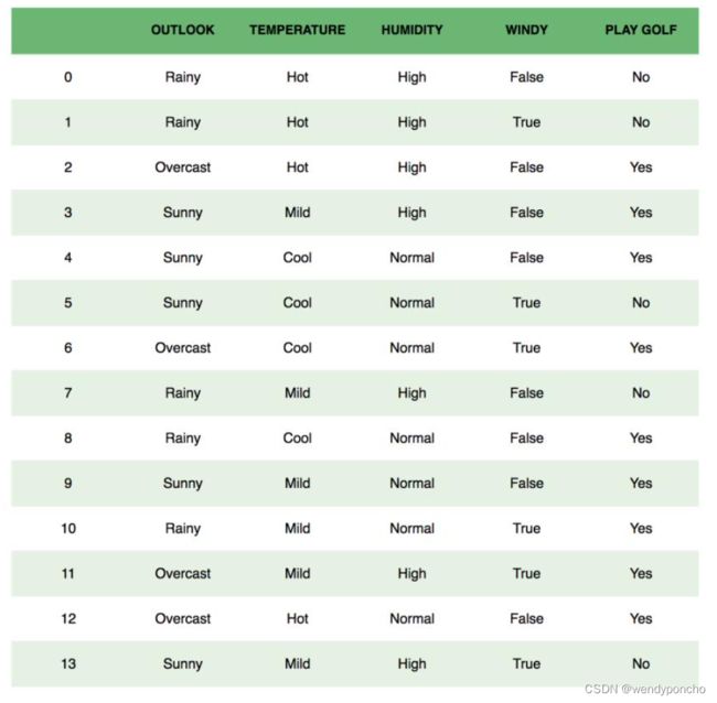
To clear, an example of a feature vector and corresponding class variable can be: (refer 1st row of the dataset)

X = (Rainy, Hot, High, False) y = No So basically, P(X|y)

here means, the probability of “Not playing golf” given that the weather conditions are “Rainy outlook”, “Temperature is hot”, “high humidity” and “no wind”.

Naive Bayes Classification

1. We assume that no pair of features are dependent. For example, the temperature being ‘Hot’ has nothing to do with the humidity, or the outlook being ‘Rainy’ does not affect the winds. Hence, the features are assumed to be independent.

2. Secondly,eachfeatureisgiventhesameweight(orimportance).Forexample,knowingt he only temperature and humidity alone can’t predict the outcome accurately. None of the attributes is irrelevant and assumed to be contributing equally to the outcome

Gaussian Naive Bayes

Continuous values associated with each feature are assumed to be distributed according to a Gaussian distribution. A Gaussian distribution is also called Normal distribution. When plotted, it gives a bell-shaped curve which is symmetric about the mean of the feature values as shown below:

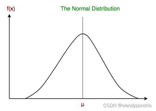
This is as simple as calculating the mean and standard deviation values of each input variable (x) for each class value.
Mean (x) = 1/n * sum(x)
Where n is the number of instances, and x is the values for an input variable in your training data.

We can calculate the standard deviation using the following equation:

Standard deviation(x) = sqrt (1/n * sum(xi-mean(x)^2 ))

Q12. What is the Confusion Matrix?

A confusion matrix is a table that is often used to describe the performance of a classification model (or “classifier”) on a set of test data for which the true values are known. It allows the visualization of the performance of an algorithm.

A confusion matrix is a table that is often used to describe the performance of a classification model (or “classifier”) on a set of test data for which the true values are known. It allows the visualization of the performance of an algorithm.

This is the key to the confusion matrix.
It gives us insight not only into the errors being made by a classifier but, more importantly, the types of errors that are being made.

Q13. What is Accuracy and Misclassification Rate?

Accuracy 

Accuracy is defined as the ratio of the sum of True Positive and True Negative by Total(TP+TN+FP+FN).

However, there are problems with accuracy. It assumes equal costs for both kinds of errors. A 99% accuracy can be excellent, good, mediocre, poor, or terrible depending upon the problem.

Misclassification Rate

Misclassification Rate is defined as the ratio of the sum of False Positive and False Negative by Total(TP+TN+FP+FN)
Misclassification Rate is also called Error Rate.

Q14. True Positive Rate & True Negative Rate

True Positive Rate:

Sensitivity (SN) is calculated as the number of correct positive predictions divided by the total number of positives.

It is also called Recall (REC) or true positive rate (TPR). The best sensitivity is 1.0, whereas the worst is 0.0.

True Negative Rate

Specificity (SP) is calculated as the number of correct negative predictions divided by the total number of negatives. It is also called a true negative rate (TNR). The best specificity is 1.0, whereas the worst is 0.0.

Q15. What is False Positive Rate & False negative Rate?

False Positive Rate

False positive rate (FPR) is calculated as the number of incorrect positive predictions divided by the total number of negatives. The best false positive rate is 0.0, whereas the worst is 1.0. It can also be calculated as 1 – specificity.

False Negative Rate

False Negative rate (FPR) is calculated as the number of incorrect positive predictions divided by the total number of positives. The best false negative rate is 0.0, whereas the worst is 1.0.

Q16. What are F1 Score, precision and recall?

Recall

Recall can be defined as the ratio of the total number of correctly classified positive examples divide to the total number of positive examples.

1. High Recall indicates the class is correctly recognized (small number of FN).

2. Low Recall indicates the class is incorrectly recognized (large number of FN).

Recall is given by the relation:

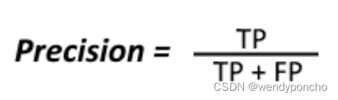
Precision

To get the value of precision, we divide the total number of correctly classified positive examples by the total number of predicted positive examples.

1. High Precision indicates an example labeled as positive is indeed positive (a small number of FP).

2. Low Precision indicates an example labeled as positive is indeed positive (large number of FP).

The relation gives precision:

Remember:
High recall, low precision: This means that most of the positive examples are correctly recognized (low FN), but there are a lot of false positives.
Low recall, high precision: This shows that we miss a lot of positive examples (high FN), but those we predict as positive are indeed positive (low FP).

F-measure/F1-Score:

Since we have two measures (Precision and Recall), it helps to have a measurement that represents both of them. We calculate an F-measure, which uses Harmonic Mean in place of Arithmetic Mean as it punishes the extreme values more.

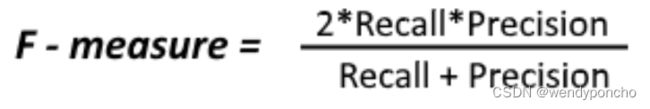The F-Measure will always be nearer to the smaller value of Precision or Recall.

Q17. What is Randomized Search CV?

Randomized search CV is used to perform a random search on hyperparameters. Randomized search CV uses a fit and score method, predict proba, decision_func, transform, etc..,
The parameters of the estimator used to apply these methods are optimized by cross-validated search over parameter settings.

In contrast to GridSearchCV, not all parameter values are tried out, but rather a fixed number of parameter settings is sampled from the specified distributions. The number of parameter settings that are tried is given by n_iter.

Q18. What is Grid Search CV?

Q19. What is Baysian Search CV?

Q20. What is ZCA Whitening?

未完待续