基于GA遗传优化的混合发电系统优化配置算法matlab仿真

目录

1.课题概述

2.系统仿真结果

3.核心程序与模型

4.系统原理简介

4.1遗传算法基本原理

4.2 混合发电系统优化配置问题

4.3 基于GA的优化配置算法

染色体编码

初始种群生成

适应度函数

选择操作

交叉操作

变异操作

5.完整工程文件

---

1.课题概述

      基于GA遗传优化的混合发电系统优化配置算法,优化风力发电，光伏发电以及蓄电池发电。

2.系统仿真结果

3.核心程序与模型

版本：MATLAB2022a

...................................................................................
[Apv,Aw,Cb,CT,LPSP,Pdump,Pdeficit,SOC,Iteration,BestJ,Bfi]=GASolveHybirdSystemSize(WindDataPV,SolarDataPVR,LoadDataPV,Apv_max,Aw_max,Cb_max);
Apv,Aw,Cb,CT,LPSP


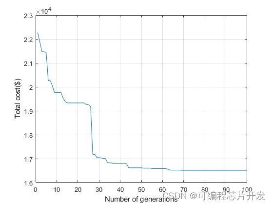
figure(1);
plot(Iteration,BestJ); 
xlabel('Number of generations');ylabel('Total cost($)');
grid on;


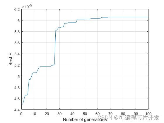
figure(2);
plot(Iteration,Bfi);
xlabel('Number of generations');ylabel('Best F');
grid on;
i=1:1:8760;


figure(3);
subplot(311);
plot(i,LoadDataPV,'r');
xlabel('Time(h)');ylabel('Load data(kW) ');
grid on;
subplot(312);
func_plot_phist(LoadDataPV,50);
xlabel('Load data(kW)');
ylabel('Percent(%)');
title('原数据概论图');
subplot(313);
func_plot_phist2(LoadDataPV,50);
xlabel('Load data(kW)');
ylabel('Percent(%)');
title('去掉两端极值后概论图');


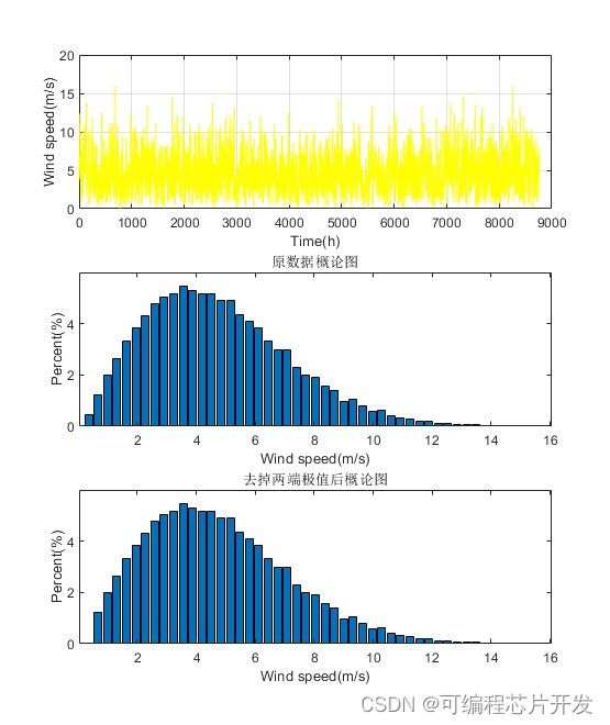
figure(4);
subplot(311);
plot(i,WindDataPV,'y');
xlabel('Time(h)');ylabel('Wind speed(m/s)');
grid on;
subplot(312);
func_plot_phist(WindDataPV,50);
xlabel('Wind speed(m/s)');
ylabel('Percent(%)');
title('原数据概论图');
subplot(313);
func_plot_phist2(WindDataPV,50);
xlabel('Wind speed(m/s)');
ylabel('Percent(%)');
title('去掉两端极值后概论图');

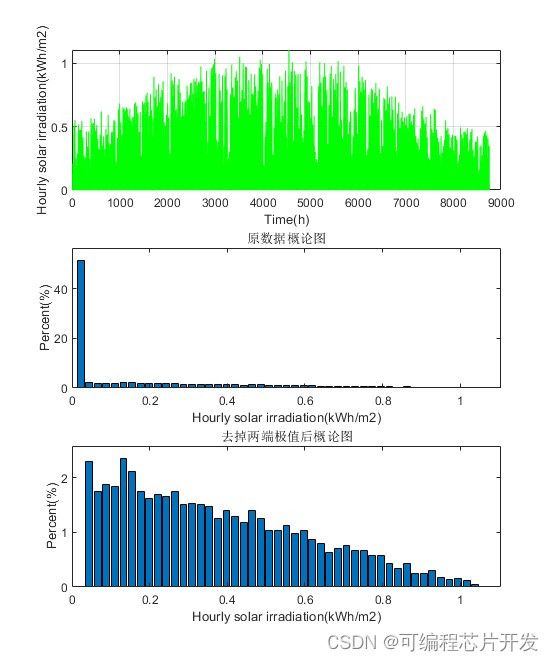
figure(5);
subplot(311);
plot(i,SolarDataPVR,'g');
xlabel('Time(h)');ylabel('Hourly solar irradiation(kWh/m2)');
grid on;
subplot(312);
func_plot_phist(SolarDataPVR,50);
xlabel('Hourly solar irradiation(kWh/m2)');
ylabel('Percent(%)');
title('原数据概论图');
subplot(313);
func_plot_phist2(SolarDataPVR,50);
xlabel('Hourly solar irradiation(kWh/m2)');
ylabel('Percent(%)');
title('去掉两端极值后概论图');

i=1:1:8760+1;
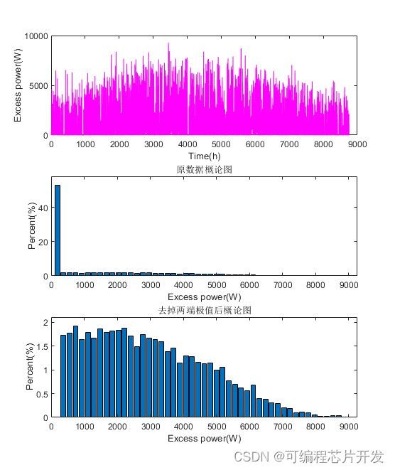
figure(6);
subplot(311);
plot(i,Pdump,'m');
xlabel('Time(h)');ylabel('Excess power(W)');
subplot(312);
func_plot_phist(Pdump,50);
xlabel('Excess power(W)');
ylabel('Percent(%)');
title('原数据概论图');
subplot(313);
func_plot_phist2(Pdump,50);
xlabel('Excess power(W)');
ylabel('Percent(%)');
title('去掉两端极值后概论图');

figure(7);
subplot(311);
plot(i,Pdeficit,'k');
xlabel('Time(h)');ylabel('Deficient power(W)');
grid on;
subplot(312);
func_plot_phist(Pdeficit,50);
xlabel('Deficient power(W)');
ylabel('Percent(%)');
title('原数据概论图');
subplot(313);
func_plot_phist2(Pdeficit,50);
xlabel('Deficient power(W)');
ylabel('Percent(%)');
title('去掉两端极值后概论图');

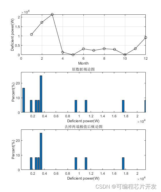
figure(8);
Pdeficit_month = zeros(floor(length(Pdeficit)/720),1);
for mm = 1:length(Pdeficit_month)
    Pdeficit_month(mm) = sum(Pdeficit(720*(mm-1)+1:720*mm));
end
j = 1:length(Pdeficit_month);
subplot(311);
plot(j,Pdeficit_month,'k-o');
xlabel('Month');ylabel('Deficient power(W)');
grid on;
subplot(312);
func_plot_phist(Pdeficit_month,50);
xlabel('Deficient power(W)');
ylabel('Percent(%)');
title('原数据概论图');
subplot(313);
func_plot_phist2(Pdeficit_month,50);
xlabel('Deficient power(W)');
ylabel('Percent(%)');
title('去掉两端极值后概论图');


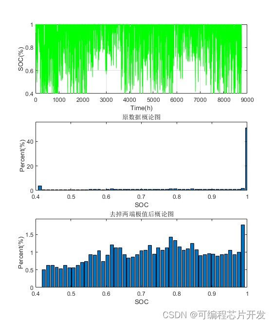
figure(9);
subplot(311);
plot(i,SOC,'g');
xlabel('Time(h)');ylabel('SOC(%)');
grid on;
subplot(312);
func_plot_phist(SOC,50);
xlabel('SOC');
ylabel('Percent(%)');
title('原数据概论图');
subplot(313);
func_plot_phist2(SOC,50);
xlabel('SOC');
ylabel('Percent(%)');
title('去掉两端极值后概论图');

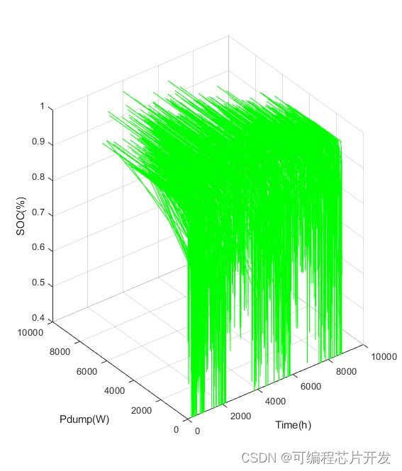
figure(10);
plot3(i,Pdump,SOC,'g');
xlabel('Time(h)');ylabel('Pdump(W)');zlabel('SOC(%)');
grid on;


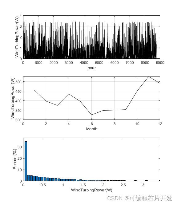
%7、画出风力发电机在这一年中产生的功率图
load WindTurbingPower.mat 
figure(11);
j = 1:length(Pw)
subplot(311);
plot(j,Pw,'k-');
xlabel('hour');ylabel('WindTurbingPower(W)');
grid on;
Pw_month = zeros(floor(length(Pw)/720),1);
for mm = 1:length(Pw_month)
    Pw_month(mm) = sum(Pw(720*(mm-1)+1:720*mm));
end
j = 1:length(Pw_month);
subplot(312);
plot(j,Pw_month,'k-');
xlabel('Month');ylabel('WindTurbingPower(W)');
grid on;
subplot(313);
func_plot_phist(Pw,50);
xlabel('WindTurbingPower(W)');
ylabel('Percent(%)');
 



%8、画出光伏发电机在这一年中产生的功率图
load SolarPower.mat 
figure(12);
j = 1:length(Ppv)
subplot(311);
plot(j,Ppv,'k-');
xlabel('hour');ylabel('SolarPower(W)');
grid on;
Ppv_month = zeros(floor(length(Ppv)/720),1);
for mm = 1:length(Ppv_month)
    Ppv_month(mm) = sum(Ppv(720*(mm-1)+1:720*mm));
end
j = 1:length(Ppv_month);
subplot(312);
plot(j,Ppv_month,'k-');
xlabel('Month');ylabel('SolarPower(W)');
grid on;
subplot(313);
func_plot_phist(Ppv,50);
xlabel('SolarPower(W)');
ylabel('Percent(%)');
 
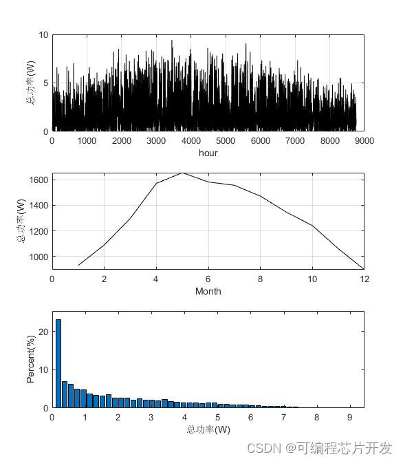
%9、画出风力发电机和光伏发电机在这一年中产生的总功率图
figure(13);
PP= Pw + Ppv;
j = 1:length(PP)
subplot(311);
plot(j,PP,'k-');
xlabel('hour');ylabel('总功率(W)');
grid on;
PP_month = zeros(floor(length(PP)/720),1);
for mm = 1:length(PP_month)
    PP_month(mm) = sum(PP(720*(mm-1)+1:720*mm));
end
j = 1:length(PP_month);
subplot(312);
plot(j,PP_month,'k-');
xlabel('Month');ylabel('总功率(W)');
grid on;
subplot(313);
func_plot_phist(PP,50);
xlabel('总功率(W)');
ylabel('Percent(%)');
02_020m

4.系统原理简介

        基于遗传算法（Genetic Algorithm, GA）的混合发电系统优化配置算法是一种通过模拟自然进化过程来求解优化问题的方法。在混合发电系统中，通常包含多种不同类型的发电单元，如风力发电、光伏发电、柴油发电机等。这些发电单元在成本、效率、可靠性等方面存在差异，因此需要通过优化配置来实现系统的经济性、可靠性和环保性等目标。

4.1遗传算法基本原理

       遗传算法是一种启发式搜索算法，它模拟了生物进化过程中的自然选择和遗传学原理。在遗传算法中，问题的解被编码成“染色体”（或称为“基因串”），每个染色体代表问题的一个潜在解。算法通过选择、交叉（杂交）和变异等操作来不断迭代优化染色体，最终找到问题的最优解或近似最优解。

4.2 混合发电系统优化配置问题

       混合发电系统的优化配置问题可以描述为：在给定的负荷需求、资源条件和技术经济参数的约束下，确定各种发电单元的最优容量配置，以最小化系统的总成本（包括投资成本、运行维护成本、燃料成本等），同时满足系统的可靠性、环保性等要求。

4.3 基于GA的优化配置算法

染色体编码

        在混合发电系统的优化配置问题中，每个染色体可以表示为一个发电单元的容量配置方案。例如，对于一个包含风力发电、光伏发电和柴油发电机的系统，染色体可以编码为 [风力发电机容量, 光伏发电容量, 柴油发电机容量]。

初始种群生成

        初始种群是遗传算法的起点，它由一定数量的随机生成的染色体组成。这些染色体代表了问题的潜在解。

适应度函数

       适应度函数用于评估染色体的优劣。在混合发电系统的优化配置问题中，适应度函数通常与系统的总成本成反比。即，成本越低的配置方案具有更高的适应度。

选择操作

        选择操作根据染色体的适应度来选择优秀的染色体进入下一代。常用的选择方法有轮盘赌选择、锦标赛选择等。

交叉操作

       交叉操作模拟了生物进化中的基因重组过程。在遗传算法中，通过交换两个染色体的部分基因来生成新的染色体。

变异操作

        变异操作模拟了生物进化中的基因突变过程。在遗传算法中，通过随机改变染色体中的某个基因来引入新的遗传信息。

       例如，对于染色体 [风力发电机容量, 光伏发电容量, 柴油发电机容量]，可以选择变异其中的光伏发电容量部分，将其替换为一个随机生成的新值。

5.完整工程文件

v

v