【目标检测】YOLOv5算法实现(四):损失计算
本系列文章记录本人硕士阶段YOLO系列目标检测算法自学及其代码实现的过程。其中算法具体实现借鉴于ultralytics YOLO源码Github,删减了源码中部分内容,满足个人科研需求。
本系列文章主要以YOLOv5为例完成算法的实现,后续修改、增加相关模块即可实现其他版本的YOLO算法。
文章地址:
YOLOv5算法实现(一):算法框架概述
YOLOv5算法实现(二):模型加载
YOLOv5算法实现(三):数据集加载
YOLOv5算法实现(四):损失计算
YOLOv5算法实现(五):预测结果后处理
YOLOv5算法实现(六):评价指标及实现
YOLOv5算法实现(七):模型训练
YOLOv5算法实现(八):模型验证
YOLOv5算法实现(九):模型预测(编辑中…)
本文目录
- 1 引言
- 2 正样本匹配
- 3 IoU计算
- 4 损失计算
1 引言
本篇文章实现模型损失函数的计算,主要涉及loss.py文件,内容包括正样本匹配和多级损失计算,其运算流程如图1所示。
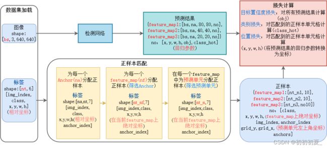
正样本匹配根据目标的实际位置,确定预测该目标的单元格位置。模型预测结果有如下形式[nf,bs,na,grid_y,grid_x,no]其中nf表示由哪几个feature_map实现对该目标的预测,na表示由哪几个Anchor实现对该目标的预测,[grid_y,grid_x]表示由哪几个像素单元实现对该目标的预测。其中feature_map上的正样本根据目标的宽高和当前feature_map上的Anchor的宽高比进行筛选,选取宽高比小于设定阈值的Anchor作为该feature_map上的样本;该feature_map上预测单元的正样本筛选如图2所示,根据目标的中心点坐标选择至多三个预测单元作为正样本。

损失计算中包含三部分损失的计算:
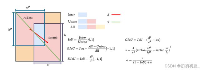
位置损失(仅计算正样本):获得正样本对应的[feature_map,img_index,anchor_index,grid_y,grid_x]的位置预测结果,和正样本计算IOU损失,不同的IOU计算方法如图3所示。Iou损失计算公式为:
I o u L o s s = 1 − I o U / G I o U / D I o U / C I o U IouLoss = 1 - IoU/GIoU/DIoU/CIoU IouLoss=1−IoU/GIoU/DIoU/CIoU
类别损失(仅计算正样本):获得正样本对应的[feature_map,img_index,anchor_index,grid_y,grid_x]的类别预测结果,和正样本计算类别损失,其中类别采用独热编码的形式[0,0,0,1,0,0],长度为目标的类别数,其中对应类别处值为1,其余位置为0。类别损失的计算方法如下:
C l s L o s s = ∑ i = 0 n f { 1 n ∑ j = 0 n [ 1 n c ∑ k = 0 k = n c ( y i log ( σ ( p i ) ) + ( 1 − y i ) log ( 1 − σ ( p i ) ) ) ] } ClsLoss = \sum\limits_{i = 0}^{nf} {\{ {1 \over n}\sum\limits_{j = 0}^n {[{1 \over {nc}}\sum\limits_{k = 0}^{k = nc} {({y_i}} } } \log (\sigma ({p_i})) + (1 - {y_i})\log (1 - \sigma ({p_i})))]\} ClsLoss=i=0∑nf{n1j=0∑n[nc1k=0∑k=nc(yilog(σ(pi))+(1−yi)log(1−σ(pi)))]}
目标类别置信度损失(计算所有样本):有正样本的位置将其值设置为IoU,其余位置设置为0。置信度损失的计算方法如下:
O b j L o s s = ∑ i = 0 n f { 1 n a ∑ j = 0 n a [ 1 g r i d y × g r i d x ∑ m = 0 g r i d y ∑ n = 0 g r i d x ( y log ( σ ( p ) ) + ( 1 − y ) log ( 1 − σ ( p ) ) ) ] } ObjLoss = \sum\limits_{i = 0}^{nf} {\{ {1 \over {na}}\sum\limits_{j = 0}^{na} {[{1 \over {gridy \times gridx}}\sum\limits_{m = 0}^{gridy} {\sum\limits_{n = 0}^{gridx} {(y\log (\sigma (p)) + (1 - y)\log (1 - \sigma (p)))]} } } } \} ObjLoss=i=0∑nf{na1j=0∑na[gridy×gridx1m=0∑gridyn=0∑gridx(ylog(σ(p))+(1−y)log(1−σ(p)))]}
2 正样本匹配
    def build_targets(self, p, targets):
        '''
        所有GT筛选相应的anchor正样本
        :param p: 预测信息(feature_map输出)
                list, 存放三个列表, 如输入为(4, 3, 640, 640)
                {[4, 3, 80, 80, 85], [4, 3, 40, 40, 85], [4, 3, 20, 20, 85]}
                [bs, na, grid_y, grid_x, xywh(回归参数)+class+classes]
        :param targets: 当前batch中的真实框 [nt, 6] [image_index, classes, xywh(相对坐标)]
        :return:tcls: 正样本类别
                tbox: 正样本位置(xywh) 其中xy为这个target对当前grid_cell左上角偏移量, xywh均为当前特征图上的绝对坐标
                indices: b:表示正样本的image index
                         a:表示正样本使用的anchor index
                         gj: 表示正样本的预测单元左上角y坐标
                         gi: 表示正样本的预测单元左上角x坐标
                anch: 表示正样本使用的anchor的尺度(相对于feature map)
        '''
        na, nt = self.na, targets.shape[0]  # anchor数量, 当前图片中的标签数
        tcls, tbox, indices, anch = [], [], [], []  # 存储类别、位置、索引、Anchor尺度

        # gain是为了后面将targets=[na, nt, t]中的相对坐标xywh映射到feature map上(绝对坐标)
        # image_index + class + xywh + anchor_index
        gain = torch.ones(7, device=self.device)

        # ai代表3个anchor上的所有target对应的anchor索引
        # [1, 3](0, 1, 2) -> [3, 1] -> [3, nt] 第一行nt个0, 第二行nt个1, 第三行nt个2
        ai = torch.arange(na, device=self.device).float().view(na, 1).repeat(1, nt)

        # 对一个feature map:这一步操作将target复制三份, 每一份对应一个feature map的一个anchor
        # 先假设所有的target的由三个anchor进行匹配, 再进行筛选, 将ai加进去用于标记当前target匹配的anchor_index
        # [nt, 6] [3, nt] -> [3, nt, 6] [3, nt, 1] -> [3, nt, 7] 7:image_index+class+xywh+anchor_index
        targets = torch.cat((targets.repeat(na, 1, 1), ai[..., None]), dim=2)

        # 以下两个参数用于扩展正样本, 一个target可能有多个cell预测到(上下左右, 3个anchor, 3个feature, 3个cell, 最多有3×3×3个anchor进行匹配)
        g = 0.5  # 中心偏移, 用于配上或下cell以及左或右cell
        # 以自身+周围上下左右4个网格 = 5个网格 来计算offsets, 最后的grid要减去偏移量
        off = torch.tensor(
            [
                [0, 0],
                [1, 0],   # j 左边(x-1)
                [0, 1],   # k 上边(y-1)
                [-1, 0],  # l 右边(x+1)
                [0, -1],  # m 下边(y+1)
            ],
            device=self.device).float() * g  # offsets
        # 遍历三个feature map, 筛选正样本
        for i in range(self.nl):  # nl: 输出特征层数量
            # 当前feature map对应的anchor尺寸 [3, 2]
            anchors, shape = self.anchors[i], p[i].shape

            # gain增益, 保存当前feature map的宽和高: gain[2:6] = gain[w, h, w, h]
            # gain用于将target上的xywh相对坐标转换为feature_map上的绝对坐标
            gain[2:6] = torch.tensor(shape)[[3, 2, 3, 2]]  # (1, 1, w, h, w, h, 1)

            t = targets * gain  # [3, nt, 7] 7:image_index + class + xywh(特征图上的绝对坐标) + anchor_index

            # 若存在正样本, 则开始匹配
            if nt:
                # t[:, :, 4:6] shape [3, nt, 2], anchors[:, None] shape[3, 1, 2]
                # r[3, nt, 2]
                # 所有的gt与当前层的三个anchor的宽高比(w / w, h / h)
                r = t[..., 4:6] / anchors[:, None]

                # 正样本筛选条件 GT与anchor的宽比或高比超过一定的阈值, 就当作负样本
                # torch.max(r, 1. / r) = [3, 63, 2] 筛选出宽比w1/w2, w2/w1和高比h1/h2, h2/h1中最大的那个
                # .max(dim=2)返回宽比、高比两者中较大的一个值和其索引, [0]为返回值, [1]为返回索引
                # j [3, nt] 小于anchor_t的为正样本 True:正样本, False:负样本
                j = torch.max(r, 1 / r).max(2)[0] < self.hyp['anchor_t']

                # 根据筛选条件j, 过滤负样本, 得到所有gt的anchor正样本
                # 知道gt的坐标属于哪张图片正样本对应的idx, 也就得到了当前正样本anchor
                # t [3, nt, 7], j[3, nt](假设其中42个为True) -> [126, 7]
                t = t[j]

                # offsets筛选当前格子周围格子, 找到两个离target中心最近的两个格子, 可能周围的格子也预测到了当前样本
                # 除了target所在的当前格子, 还有2个格子对目标进行检测(计算损失)
                # 利用中心坐标对1求余与g比较, 判断选择哪两个格子
                # gxy:[126, 2] gain[[2, 3]]:[1,2]
                gxy = t[:, 2:4]  # grid xy 取目标中心的坐标(绝对坐标,相对于feature map左上角的坐标)
                gxi = gain[[2, 3]] - gxy  # (绝对坐标, 相对于feature map右下角的坐标)

                # j: [126] 如果是True表示当前target中心点所在的格子的左边格子也对该target进行回归
                # k: [126] 如果是True表示当前target中心点所在大的格子的上边格子也对该target进行回归
                j, k = ((gxy % 1 < g) & (gxy > 1)).T

                # l: [126] 如果是True表示当前target中心点所在的格子的右边格子也对该target进行回归
                # m: [126] 如果是True表示当前target中心点所在的格子的下边格子也对该target进行回归
                l, m = ((gxi % 1 < g) & (gxi > 1)).T

                # j [5, 126] torch.ones_like(j): 当前格子不需要筛选均为True, j,k,m,l:左上右下格子的筛选结果
                j = torch.stack((torch.ones_like(j), j, k, l, m))
                # 得到筛选后的所有格子正样本 格子数 <= 3 * 126, 不在边上时等号成立
                # t复制5份, 分别对应五个格子
                # t [126, 7]->[5, 126, 7]; j[5, 126]
                # t[5, 126, 7] + j[5, 126] = t[378, 7] 理论上小于等于3倍的126, 当且仅当没有边界格子时等号成立
                t = t.repeat((5, 1, 1))[j]

                # gxy:[126, 2] torch.zeros_like(gxy)[None]: [1, 126, 2]
                # off:[5,2]  off[:, None]:[5, 1, 2]  off[:, None][j] = [5, 126, 2] + [5, 126] = [378, 2] 广播机制
                # offsets: [378, 2]得到所有筛选后的网格的中心相对于这个要预测的真实框所在网格边界(左右上下边框)的偏移量
                offsets = (torch.zeros_like(gxy)[None] + off[:, None])[j]
            else:
                t = targets[0]
                offsets = 0
            # t[378, 7] t.chunk(4, dim=1)在维度1上划分为4个块 (image_index, class, x, y, w, h, anchor_index)
            # bc:(image_index, class) gxy gwh a(anchor_index)
            bc, gxy, gwh, a = t.chunk(4, 1)
            # a:anchor_index, b:image_index, c:class
            a, (b, c) = a.long().view(-1), bc.long().T
            gij = (gxy - offsets).long()  # 预测真实框的网络所在的左上角坐标, 其中.long()化为长整型进行了取整 [378, 2]
            gi, gj = gij.T  # grid xy

            # b:image_index, a:anchor_index, gj:网格左上角y坐标, gi:网格的左上角x坐标
            indices.append((b, a, gj.clamp_(0, shape[2] - 1), gi.clamp_(0, shape[3] - 1)))
            # xywh(绝对坐标), 其中xy为target对当前grid_cell左上角的偏移量
            tbox.append(torch.cat((gxy - gij, gwh), 1))
            # 对应所有的anchors
            anch.append(anchors[a])
            tcls.append(c)

        return tcls, tbox, indices, anch
3 IoU计算
def bbox_iou(box1, box2, xywh=True, GIoU=False, DIoU=False, CIoU=False, eps=1e-7):
    '''
    计算Iou/GIou/DIou/CIou,默认计算普通IoU
    '''

    # 将xywh坐标形式转换成xyxy(左上角右下角)坐标形式,便于计算面积与对角线长度
    if xywh:  # transform from xywh to xyxy
        (x1, y1, w1, h1), (x2, y2, w2, h2) = box1.chunk(4, -1), box2.chunk(4, -1)
        w1_, h1_, w2_, h2_ = w1 / 2, h1 / 2, w2 / 2, h2 / 2
        b1_x1, b1_x2, b1_y1, b1_y2 = x1 - w1_, x1 + w1_, y1 - h1_, y1 + h1_
        b2_x1, b2_x2, b2_y1, b2_y2 = x2 - w2_, x2 + w2_, y2 - h2_, y2 + h2_
    else:  # x1, y1, x2, y2 = box1
        b1_x1, b1_y1, b1_x2, b1_y2 = box1.chunk(4, -1)
        b2_x1, b2_y1, b2_x2, b2_y2 = box2.chunk(4, -1)
        w1, h1 = b1_x2 - b1_x1, b1_y2 - b1_y1 + eps
        w2, h2 = b2_x2 - b2_x1, b2_y2 - b2_y1 + eps

    # 计算交集面积
    inter = (torch.min(b1_x2, b2_x2) - torch.max(b1_x1, b2_x1)).clamp(0) * \
            (torch.min(b1_y2, b2_y2) - torch.max(b1_y1, b2_y1)).clamp(0)

    # 计算并集面积
    union = w1 * h1 + w2 * h2 - inter + eps

	# 计算IoU
    iou = inter / union
    if CIoU or DIoU or GIoU:
    	# 计算包围两个矩形框的最小框宽和高
        cw = torch.max(b1_x2, b2_x2) - torch.min(b1_x1, b2_x1)  # 最小包围矩形框宽度
        ch = torch.max(b1_y2, b2_y2) - torch.min(b1_y1, b2_y1)  # 最小包括矩形框高度
        if CIoU or DIoU:  # Distance or Complete IoU https://arxiv.org/abs/1911.08287v1
            c2 = cw ** 2 + ch ** 2 + eps  # 最小包围矩形框对角线长度
            rho2 = ((b2_x1 + b2_x2 - b1_x1 - b1_x2) ** 2 + (b2_y1 + b2_y2 - b1_y1 - b1_y2) ** 2) / 4  # 矩形框中心点连线长度
            if CIoU:  # https://github.com/Zzh-tju/DIoU-SSD-pytorch/blob/master/utils/box/box_utils.py#L47
                v = (4 / math.pi ** 2) * torch.pow(torch.atan(w2 / h2) - torch.atan(w1 / h1), 2)
                with torch.no_grad():
                    alpha = v / (v - iou + (1 + eps))
                return iou - (rho2 / c2 + v * alpha)  # CIoU
            return iou - rho2 / c2  # DIoU
        c_area = cw * ch + eps  # 最小包围矩形框面积
        return iou - (c_area - union) / c_area  # GIoU https://arxiv.org/pdf/1902.09630.pdf
    return iou  # IoU
4 损失计算
class ComputeLoss:
    '''
    Anchor-based
    YOLOv5正负样本匹配方法
    '''
    sort_obj_iou = False  # 后面筛选置信度损失时是否先对iou进行排序
    def __init__(self, model):
        device = next(model.parameters()).device  # 获取模型训练的设备
        h = model.hyp  # 损失计算中用到的超参数

        # 定义obj置信度损失和分类损失
        # 其中pos_weight为了处理样本不均衡问题, 在正样本的损失前面乘上系数
        BCEcls = nn.BCEWithLogitsLoss(pos_weight=torch.tensor([h['cls_pw']], device=device))
        BCEobj = nn.BCEWithLogitsLoss(pos_weight=torch.tensor([h['obj_pw']], device=device))

        # 标签平滑, 防止过拟合并能缓解分类问题中错误标签的影响
        # 正样本标签, 负样本标签
        self.cp, self.cn = smooth_BCE(eps=h.get('label_smoothing', 0.0))


        m = model.model[-1]  # Detect() module
        # 针对obj损失, 对samll, medium, large物体的检测损失乘上系数
        self.balance = {3: [4.0, 1.0, 0.4]}.get(m.nl, [4.0, 1.0, 0.25, 0.06, 0.02])

        self.BCEcls, self.BCEobj, self.hyp = BCEcls, BCEobj, h
        self.na = m.na  # anchors数量
        self.nc = m.nc  # 类别数量
        self.nl = m.nl  # 输出特征层数量
        self.anchors = m.anchors  # anchors [3, 3, 2], 缩放到feature map上的anchors尺寸
        self.device = device
    def __call__(self, p, targets):  #predictions, targets
        # prediction ([bs, 3, 20, 20, 85], [bs, 3, 40, 40, 85], [bs, 3, 80, 80, 85])
        # targets[nt, 6]  image_index, classes, xywh
        lcls = torch.zeros(1, device=self.device)  # 类别损失
        lbox = torch.zeros(1, device=self.device)  # 位置损失
        lobj = torch.zeros(1, device=self.device)  # 物体置信度损失
        # 正样本匹配: 根据实际目标(x, y)筛选正样本grid, 根据实际目标(w, h)和anchors的长宽比筛选用于匹配的anchor
        # tcls: 正样本类别 tbox: 正样本在当前feature map上的绝对坐标 xywh, 其中xywh为相对grid_cell左上角偏移量
        # indices: image_index, anchor_index, gj, gi anchors: target使用的anchor尺度(相对于feature map)
        tcls, tbox, indices, anchors = self.build_targets(p, targets)  # targets

        # 计算损失, 针对每一个feature_map进行
        for i, pi in enumerate(p):  # 层数, 预测信息[bs, 3, 20, 20, 85]
            # 当前正样本的匹配信息: image_index, anchor_index, gridy, gridx
            b, a, gj, gi = indices[i]
            # 目标置信度(初始化为0)
            tobj = torch.zeros(pi.shape[:4], dtype=pi.dtype, device=self.device)  # [bs, 3, 20, 20]
            # 当前预测feature_map上的匹配正样本数
            n = b.shape[0]
            if n:  # 若存在正样本
                # 对应的正样本预测信息 xy:[nt, 2], wh:[nt, 2], cls[nt, nc]
                pxy, pwh, _, pcls = pi[b, a, gj, gi].split((2, 2, 1, self.nc), dim=1)

                # 预测的回归参数进行回归到feature_map上的xy绝对坐标
                pxy = pxy.sigmoid() * 2 - 0.5
                # 预测的回归参数进行回归到feature_map上的wh绝对坐标
                # anchors[i]当前匹配的正样本的anchors尺寸, 对应feature map
                pwh = (pwh.sigmoid() * 2) ** 2 * anchors[i]
                # 预测的边界框, 相对于feature map的绝对值(xy为相对cell的)
                pbox = torch.cat((pxy, pwh), 1)
                # 计算IoU
                iou = bbox_iou(pbox, tbox[i], CIoU=True).squeeze()
                # 计算IoU损失
                lbox += (1.0 - iou).mean()

                iou = iou.detach().clamp(0).type(tobj.dtype)
                if self.sort_obj_iou:  # 根据iou对正样本进行排序
                    j = iou.argsort()
                    b, a, gj, gi, iou = b[j], a[j], gj[j], gi[j], iou[j]
                # 利用iou作为物体置信度的标签值
                tobj[b, a, gj, gi] = iou

                # 计算分类损失, 若nc=1, 则类别损失与物体置信度损失重复, 无需重复计算
                if self.nc > 1:
                    # 负样本标签为cn
                    t = torch.full_like(pcls, self.cn, device=self.device)
                    # 正样本标签为cp
                    t[range(n), tcls[i]] = self.cp
                    lcls += self.BCEcls(pcls, t)
            # 计算物体置信度损失, 针对所有样本
            obji = self.BCEobj(pi[..., 4], tobj)
            # 针对不同大小的feature map即针对不同大小的物体检测的损失权重不同
            lobj += obji * self.balance[i]

        lbox *= self.hyp['box']
        lobj *= self.hyp['obj']
        lcls *= self.hyp['cls']

        # loss = lbox + lobj + lcls
        return {"box_loss": lbox,
                "obj_loss": lobj,
                "class_loss": lcls}
    def build_targets(self, p, targets):
		pass