【图像拼接】源码精读：Quality evaluation-based iterative seam estimation for image stitching

第一次来请先看这篇文章：【图像拼接（Image Stitching）】关于【图像拼接论文源码精读】专栏的相关说明，包含专栏内文章结构说明、源码阅读顺序、培养代码能力、如何创新等（不定期更新）

【图像拼接论文源码精读】专栏文章目录

1. 【源码精读】As-Projective-As-Possible Image Stitching with Moving DLT（APAP）第一部分：全局单应Global homography
2. 【图像拼接】源码精读：Seam-guided local alignment and stitching for large parallax images

---

前言

论文题目：Quality evaluation-based iterative seam estimation for image stitching - 基于质量评估的迭代接缝估计图像拼接方法

论文链接：Quality evaluation-based iterative seam estimation for image stitching

论文源码：https://github.com/tlliao/Iterative-seam-estimation

注：matlab源码，相关算法是C++封装的。主要是对matlab的学习与理解。

【图像拼接论文精读】专栏对应文章：【图像拼接】论文精读：Quality evaluation-based iterative seam estimation for image stitching

配合对应的文章阅读，效果更佳！

注：请重点关注代码段中的注释！！！有一些讲解的东西直接写在代码段的注释中了，同时多关注红色字体和绿色字体！！！

1. 跑通代码，得到结果

任何源码下载下来后，第一件事就是先跑通。

无论你是否要在该工作的基础上创新，总是需要得到拼接结果，在论文的实验部分做对比。

所以，请务必跑通，得到拼接结果。

1.1 准备工作

本地需要matlab环境，我是MATLAB R2018b，选择一个适中的matlab版本即可。（最新的matlab2023可以使用局部函数了，类似jupyter notebook，感兴趣的同学可以试试最新版。）

源码下载下来后，用matlab打开项目，界面如下：

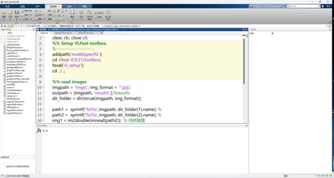
左侧是文件目录结构，中级是当前所选文件代码，下面是命令行窗口，右侧是工作区（运行后显示相关变量的值）

1.2 尝试运行

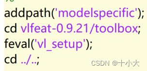
点击上面菜单栏【运行】，出现如下报错：

检查后发现，当前目录下为vlfeat-0.9.21文件夹，而不是vlfeat-0.9.20。修改为：

并将其他源码中的vlfeat-0.9.21文件夹复制过来。初始下载的源码中vlfeat-0.9.21为空。

如果在其他论文源码中找不到可用的vlfeat-0.9.21，则可以直接点击下面的链接下载。

vlfeat-0.9.21下载链接（已经配置好，复制到源码目录下可以直接使用）：图像拼接论文源码matlab所需的vlfeat-0.9.21库，已经配置好，复制到源码目录下即可直接使用

除此之外，文件目录下还缺少Imgs文件夹。将其添加，这里以temple数据集为例，目录变为下图所示：

此时运行代码，已经可以完整的跑通了。

1.3 得到拼接结果

跑通的命令行显示与拼接结果：

这里我互换了参照图和目标图，让右图为目标图。

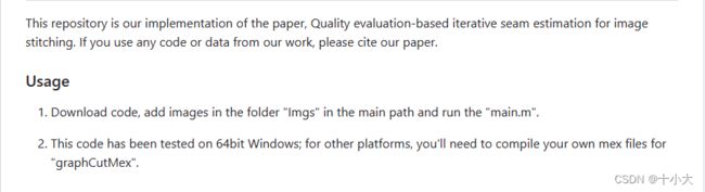
附上原作者README中的使用方法：

2. 源码解读，看懂原理

本节将按照main.m中的代码顺序进行【模块化】讲解，包括与论文中的算法对应、matlab语法和函数学习、变量的类型和值、函数功能等方面。代码段中包含原作者的注释和我做的注释，与讲解结合着阅读。

2.1 准备工作

代码如下：

clear; clc; close all; 
%% Setup VLFeat toolbox.
%----------------------
addpath('modelspecific'); 
cd vlfeat-0.9.21/toolbox;
feval('vl_setup');
cd ../..;

%% read images
imgpath = 'Imgs\'; img_format = '*.jpg';
outpath = [imgpath, 'results\'];%results
dir_folder = dir(strcat(imgpath, img_format));

path1 =  sprintf('%s%s',imgpath, dir_folder(1).name); %
path2 =  sprintf('%s%s',imgpath, dir_folder(2).name); %
img1 = im2double(imread(path2));  % 待拼接图
img2 = im2double(imread(path1));  % 基准图

代码包含重复运行的清空操作，设置vlfeat库，读取Imgs文件夹下的输入图像，得到两张输入图像img1和img2。这里我们将参照图和目标图互换，右图为目标图，符合其他论文将右图作为目标图的习惯。

2.2 提取特征匹配点并对齐图像

代码如下：

%% detect features and align images
fprintf('> feature matching and image alignment...');tic;
[warped_img1, warped_img2] = registerTexture(img1, img2);
fprintf('done (%fs)\n', toc);    

registerTexture函数：

function [warped_img1, warped_img2] = registerTexture(img1, img2)
% given two images, detect sift feature matches and calculate the homography warp
% img1: target image to be warped
% img2: reference image
% warped_img1: warped img1
% warped_img2: warped img2

[pts1, pts2] = siftMatch(img1, img2); % sift feature matches
Sz1 = max(size(img1,1),size(img2,1)); % to avoid the two images have different size
Sz2 = max(size(img1,2),size(img2,2));
[matches_1, matches_2] = matchDelete(pts1, pts2, Sz1, Sz2); % delete wrong match features (outliers)

init_H = calcHomo(matches_1, matches_2);  % fundamental homography

[warped_img1, warped_img2] = homographyAlign(img1,img2,init_H); % warped images via homography warp

end

2.2.1 总体流程

首先，sift提取到特征点（siftMatch.m），特征点pts1和pts2是2×n的非齐次格式，如果两张图像不一样大，则取最大的作为宽（Sz1）高（Sz2）。然后，筛选匹配点（matchDelete.m）得到正确匹配matches_1和matches_2，进而根据正确匹配点得到单应矩阵H（calcHomo.m）。最后，根据H对齐两张图像（homographyAlign.m），得到翘曲后的两张图像warped_img1和warped_img2。

2.2.2 matchDelete函数

• 函数功能：剔除异常值，分为【剔除重复值】、【直方图剔除离群值】和【RANSAC剔除异常值】三步。
• 参数：pts1, pts2, height, width分别为SIFT得到的两组非齐次匹配点，图像的高、宽
• 返回值：matches1, matches2剔除异常值后的正确匹配点

剔除重复值：

%% delete the wrong matches (one-to-more)
[~, ind_1] = unique(pts1', 'rows'); % pts1变成n*2，找唯一的行，返回n*1的索引
pts1 = pts1(:,ind_1');  % 保留索引，剔除重复的
pts2 = pts2(:,ind_1');
[~, ind_2] = unique(pts2', 'rows'); % 从pst2中再剔除重复的
pts1 = pts1(:,ind_2');
pts2 = pts2(:,ind_2');

直方图剔除离群值：

%% use histogram (horizontal and vertical orientation) delete outliers
% 直方图剔除异常值

thr = 0.1;  % 划分范围，1/10，-10~+10，宽是730，则xbins间距就是73
% horizontal histogram
xbins = (-width+width*thr/2:width*thr:width-width*thr/2);   % 横坐标列表
counts1 = hist(pts1(1,:)-pts2(1,:), xbins); % 横坐标插值的直方图，个数
[~,ia1] = max(counts1); % 直方图峰值索引
% 筛选出有效范围内的横坐标插值索引（>=的是下界，<=的是上界）
% 要与最大索引所在段的相邻两段，比如ia1=7，就是要第6，7，8三段内的点
C1 = find(pts1(1,:)-pts2(1,:)>=max(-width,-width+(ia1-2)*width*thr) & pts1(1,:)-pts2(1,:)<=min(width,-width+(ia1+1)*width*thr));

% vertical histogram
ybins = (-height+height*thr/2: height*thr: height-height*thr/2);
counts2 = hist(pts1(2,:)-pts2(2,:), ybins);
[~, ia2] = max(counts2);
C2 = find(pts1(2,:)-pts2(2,:)>=max(-height,-height+(ia2-2)*height*thr) & pts1(2,:)-pts2(2,:)<=min(height, -height+(ia2+1)*height*thr));
% final inliers after 1st filter
C = intersect(C1,C2);   % 交集
pts1 = pts1(:,C);
pts2 = pts2(:,C); 

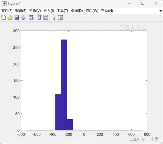
首先根据阈值thr划分间距范围，得到横纵坐标的列表，然后根据两组匹配点的差值画出直方图：

水平方向（横坐标）：

纵坐标方向：

以水平方向为例，count1的统计结果如下：
最多的点分布在第七段（ia1=7），筛选条件就是得到最大段相邻的两段，即本例中的6、7、8段，其他段内的点视为离群点。

RANSAC剔除异常值：

%% RANSAC delete
fprintf('> do RANSAC feature filter...\n');tic;
coef.minPtNum = max(min(round(size(pts1,2)/4),10),4);
coef.iterNum = 1000;
coef.thDist = 5;
coef.thInlrRatio = .1;
 

[~,corrPtIdx1] = ransacx(pts1, pts2, coef); 
matches1 = pts1(:, corrPtIdx1);
matches2 = pts2(:, corrPtIdx1);

其中，ransacx函数是执行ransac过程，找到内点最多的模型

function [f,inlierIdx] = ransacx( x,y, ransacCoef )%, funcFindF, funcDist)
% 函数功能：使用RANSAC，找到从x到y的拟合
% x，y：n个点的矩阵，维数×n。本例就是2×n

% ransacCoef：参数结构体，包含四个字段minPtNum,iterNum,thDist,thInlrRatio，其中
% minPtNum：找到拟合点的最小点数，直线拟合是2，单应是4
% iterNum：迭代次数
% thDist：离群点距离阈值
% thInlrRatio：内点阈值比例

% f，inlierIdx：返回拟合结果和内点索引

minPtNum = ransacCoef.minPtNum; 
iterNum = ransacCoef.iterNum;
thInlrRatio = ransacCoef.thInlrRatio;
thDist = ransacCoef.thDist;

ptNum = size(x,2);
thInlr = round(thInlrRatio*ptNum);  % 内点数量阈值

inlrNum = zeros(1,iterNum);
fLib = cell(1,iterNum);

% 执行RANSAC过程
% 1. 随机选择minPtNum个点，计算单应变换
% 2. 计算选择的点到模型的距离，找到符合阈值条件thDist的内点inlier1
% 3. 如果内点数小于thInlr，则继续迭代
% 4. 选择内点最多的模型索引 idx 和数量 max_inlier
% 如果最大内点数量为零，则返回空值。
% 否则，使用具有最大内点数量的模型重新计算几何模型 f，并标识出距离模型距离小于 thDist 的内点索引 inlierIdx
parfor p = 1:iterNum
	% 1. fit using  random points 
	sampleIdx = randIndex(ptNum,minPtNum);
	f1 = calcHomo(x(:,sampleIdx),y(:,sampleIdx));%funcFindF(x(:,sampleIdx),y(:,sampleIdx));    % For homography: f1 is H
	
	% 2. count the inliers, if more than thInlr, refit; else iterate
	dist = calcDist(f1,x,y);%funcDist(f1,x,y);
	inlier1 = find(dist < thDist);      %caculate count of inlier
	if length(inlier1) < thInlr, continue; end
    inlrNum(p) = length(inlier1);
    fLib{p} = inlier1;  % re-caculate H
end

% 3. choose the coef with the most inliers
[max_inlier, idx] = max(inlrNum);  
if max_inlier==0
    inlierIdx = [];
    f = [];
    return;
end

f = calcHomo(x(:,fLib{idx}),y(:,fLib{idx}));       %most inliers
dist = calcDist(f,x,y);     % find match point
inlierIdx = find(dist < thDist);
f = calcHomo(x(:,inlierIdx),y(:,inlierIdx));

	
end

RANSAC过程更多的细节可以查看图像拼接】源码精读：Seam-guided local alignment and stitching for large parallax images的章节2.2.3。

至此，内点inliers已经筛选完毕。

2.2.3 calcHomo函数

函数功能：根据inliers计算单应矩阵

function H = calcHomo(pts1,pts2)
%% use Direct linear tranformation (DLT) to calculate homography
%  approxmation: H*[pts1; ones(1,size(pts1,2))] = [pts2; ones(1,size(pts2,2))]
% Normalise point distribution.
data_pts = [ pts1; ones(1,size(pts1,2)) ; pts2; ones(1,size(pts2,2)) ];
[ dat_norm_pts1,T1 ] = normalise2dpts(data_pts(1:3,:));
[ dat_norm_pts2,T2 ] = normalise2dpts(data_pts(4:6,:));
data_norm = [ dat_norm_pts1 ; dat_norm_pts2 ];

%-----------------------
% Global homography (H).
%-----------------------
%fprintf('DLT (projective transform) on inliers\n');
% Refine homography using DLT on inliers.
%fprintf('> Refining homography (H) using DLT...');
[ h,~,~,~ ] = feval('homography_fit',data_norm);
H = T2\(reshape(h,3,3)*T1);

end

这里不过多赘述，与APAP中的代码基本一致。链接：【源码精读】As-Projective-As-Possible Image Stitching with Moving DLT（APAP）第一部分：全局单应Global homography

2.2.4 homographyAlign函数

函数功能：根据单应矩阵得到翘曲后的两张图像。

此处代码略，可以查看图像拼接】源码精读：Seam-guided local alignment and stitching for large parallax images的章节2.2.5。

2.3 迭代接缝估计，blendTexture函数

2.3.3对应论文的2.1部分Conventional seam-cutting，是Perception-based-seam-cutting论文中基于感知的接缝算法得到的初始接缝，通过数据项和平滑项，经过图割和梯度融合得到拼接结果。

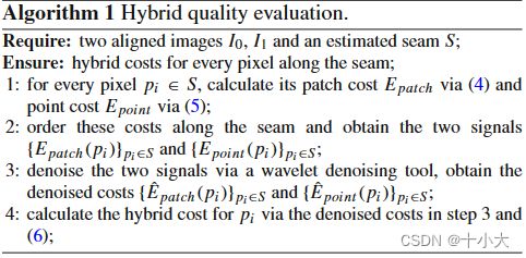
2.3.4对应论文的2.2.1 Hybrid quality evaluation和算法1，提出接缝上像素点和像素块的混合质量评估，通过小波去噪平滑信号。对应图2的展示，单独像素点成本和去噪成本、单独的像素块成本和去噪成本、点、块去噪成本和混合成本，可以看到混合的成本更低。

2.3.5对应论文的2.2.2 Seam estimation refinement和算法2，迭代优化接缝评估，根据混合评估更新差异图，错位的地方惩罚加重，两侧扩展5像素。根据新的差异图重新计算能量函数，不停地迭代更新，直到达到合理范围（差异的点少于10个，这个参数可以修改）。

main.m中的代码如下：

%% iterative seam estimation
fprintf('> seam estimation and image blending...');tic;
blendTexture(warped_img1, warped_img2);
fprintf('done (%fs)\n', toc);

本节我们将一段一段讲解blendTexture.m文件下对应的代码，也是本论文的核心。

2.3.1 参数初始化

代码如下：

 %% preparation: parameter initialization
    patchsize = 21; % the size of patch for seam evaluation
    max_iterations = 1000; % maximum iterations for seam estimation
    gray1 = rgb2gray(warped_img1);  gray2 = rgb2gray(warped_img2);  
    square_SE = strel('square', 2);
    signal_mu = 0.12;   %parameters for f(x)=exp(sigma_ratio*(x-mu))  论文中公式（7）
    sigma_ratio = 5;

设置了20×20大小的块，迭代最大次数为1000，论文中公式(7)对应的参数。

2.3.2 seam-cutting的准备工作

代码如下：

 %%  pre-process of seam-cutting
    w1 = imfill(imbinarize(gray1, 0),'holes');
    w2 = imfill(imbinarize(gray2, 0),'holes');
    A = w1;  B = w2;
    C = A & B;  % overlapping region
    [sz1, sz2] = size(C);
    ind = find(C);  % 重叠区域非零元素索引
    nNodes = size(ind,1);   % 非零像素个数
    revindC = zeros(sz1*sz2,1);
    revindC(C)=1:length(ind);
    
    [tmp_y, tmp_x] = find(B==1);
    % 目标图坐标范围，因为我们将参照图和目标图互换了
    B_x0 = tmp_x(1); B_y0 = tmp_y(1);  % begining coordinates of reference in final canvas
    B_x1 = tmp_x(end); B_y1 = tmp_y(end); % ending coordinates of reference in final canvas
    
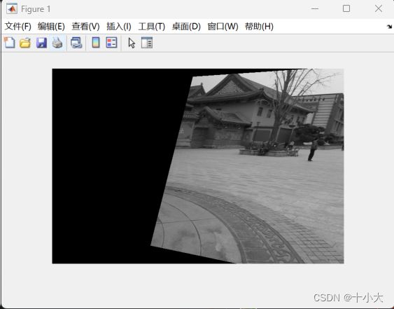
    gray_cut1 = gray1(B_y0:B_y1,B_x0:B_x1); % 灰色目标图
    gray_cut2 = gray2(B_y0:B_y1,B_x0:B_x1); % 灰色参照图
    C_cut = C(B_y0:B_y1,B_x0:B_x1); % 目标图中重叠区域掩码

gray_cut1 、gray_cut2、C_cut的可视化如下：

2.3.3 数据项、平滑项、图割

代码略。详细请见文章【图像拼接】源码精读：Seam-guided local alignment and stitching for large parallax images的2.3.1、2.3.3、2.2.4部分。

与Seam-guided local alignment and stitching for large parallax images中不同，本文方法的平滑项用的是欧式准则，而Seam-guided local alignment and stitching for large parallax images用的sigmoid。

2.3.4 评估当前接缝（本文核心，对应论文2.2.1部分）

本节对应论文中2.2.1 Hybrid quality evaluation与算法1，和部分2.2.2 Seam estimation refinement的内容。

代码段如下：

    %% evaluate the current stitching seam
    B_contour = Bs(B_y0:B_y1,B_x0:B_x1);    % 轮廓，值为1是原目标图，值为0是翘曲后的部分，1和0分界的地方是接缝
    [hybrid_signal, boundarypts] = seamRefining(gray_cut1, gray_cut2, imgdif_cut, C_cut, B_contour, patchsize);
    Boundpts = boundarypts + repmat([B_y0-1,B_x0-1],length(boundarypts),1); % 全尺寸下缝合线坐标
    [extend_signal, extendpts] = signalExtend(hybrid_signal, Boundpts, As, Bs, C);	% 扩展区域，每侧扩充5像素。

B_contour ：

seamRefining：

function [ hybrid_signal, boundarypts ] = seamRefining( gray1, gray2, imgdif, C, B_contour, patchsize)
% given seam information, calculate the patch/pixel signals and denoised
% hybrid signal, return the output signal and extend seam points

% 接缝优化
% gray1 和 gray2：两个灰度图像。
% imgdif：图像差异信息。
% C：重叠区域的二值图像。
% B_contour：轮廓信息。
% patchsize：补丁（patch）的大小。


B_seam = B_contour;
if sum(B_seam(1:end, 1))==size(B_seam,1)    % 检查第一列如果全是1，则参照图在左边，取反
    B_seam = ~B_seam;   %% to find out the reference is on the left or right
    B_seam = imdilate(imerode(B_seam, strel('square', 2)), strel('square', 2)); % 腐蚀膨胀
else
    B_seam = imdilate(imerode(B_seam, strel('square', 2)), strel('square', 2));
end

% 检查 B_seam 的第一列和第一行是否全为零，以确定是否需要对 B_seam 进行旋转。
if sum(B_seam(1:end,1)) + sum(B_seam(1,1:end))==0
    rotate_B_seam = B_seam(1+size(B_seam,1)-1:-1:1+size(B_seam,1)-end, 1+size(B_seam,2)-1:-1:1+size(B_seam,2)-end);
    boundarypts = contourTracingofRight(~rotate_B_seam);
    boundarypts = [1+size(B_seam,1)-boundarypts(:,1), 1+size(B_seam,2)-boundarypts(:,2)];
else
    boundarypts = contourTracingofRight(B_seam);    % 找到接缝边界，n×2
end
    
patch_signal = evalSeamofSSIM(gray1, gray2, C, boundarypts, patchsize); % patch signal
pixel_signal = evalSeamofPixel(imgdif, B_seam, boundarypts); % pixel signal

denoise_patch_signal = signalDenoise(patch_signal);  % denoise patch signal
denoise_pixel_signal = signalDenoise(pixel_signal);  % denoise pixel signal
hybrid_signal = 10.*denoise_patch_signal.*denoise_pixel_signal;  % hybrid signal

end

首先找到拼接缝的像素点坐标（考虑参照图在左还是在右，是否旋转过），对接缝上每个像素点，定义一个块（20×20），计算这个局部块的SSIM。如果SSIM为1，则认为两个块相同，不需要优化。将像素块和像素点作为一个混合的去噪成本，后续优化它。定义为论文中的公式（6）：

通过源码我们得知，$\lambda =10$。

关于去噪方式：作者尝试过高斯滤波平滑和小波平滑，最后发现小波去噪更有效。

2.2.5 迭代接缝评估优化（文本核心，对应论文2.2.2部分）

按公式（7）修改接缝上未对齐接缝像素的成本：

%% 2nd-iteration for further refinement        
    % calculate a new stitching seam
    imgdif2 = imgdif;  ind_seam = (extendpts(:,2)-1)*sz1 + extendpts(:,1);
    imgdif2(ind_seam) = imgdif2(ind_seam).*(exp(sigma_ratio.*(extend_signal-signal_mu))); %公式（7）
    DL = (imgdif2(CL1) + imgdif2(CL2))./2;
    DU = (imgdif2(CU1) + imgdif2(CU2))./2;
    edgeWeights2=[
        revindC(CL1) revindC(CL2) DL+1e-8 DL+1e-8;
        revindC(CU1) revindC(CU2) DU+1e-8 DU+1e-8
    ];

    %% graph cut optimization
    [~, labels2] = graphCutMex(terminalWeights, edgeWeights2);  
    
    As=A;  Bs=B;
    As(ind(labels2==1))=false;   
    Bs(ind(labels2==0))=false;   
    
    final_As = As;  

注：如果你先看了Seam-guided local alignment and stitching for large parallax images，就会发现，本文的公式（7）已经变成sigmoid了。

接缝两侧扩展5个像素生成块，设置新的混合成本，差分图重新计算，用新的差分图重新计算能量函数，迭代平滑项：

%% evaluate the current stitching seam
    B_contour = Bs(B_y0:B_y1,B_x0:B_x1); 
    [hybrid_signal2, boundarypts2] = seamRefining(gray_cut1, gray_cut2, imgdif_cut, C_cut, B_contour, patchsize);
    Boundpts2 = boundarypts2 + repmat([B_y0-1,B_x0-1], length(boundarypts2),1); % 全尺寸下缝合线坐标
    [extend_signal2, extendpts2] = signalExtend(hybrid_signal2, Boundpts2, As, Bs, C);
           
    %% iteration (while-loop) for seam refining
    end_seam = union(extendpts, extendpts2, 'rows');    % 扩展接缝
    overlap_pts = setdiff(Boundpts2, extendpts, 'rows');    % 差集
    k_seam = 3;  
    % 扩展前后的点大于10个并且迭代次数小于设置的最大迭代次数时，继续迭代
    % 1. 根据当前的接缝扩展点extendpts2来更新平滑项
    % 2. 图割得到新的接缝结果
    % 3. 最后更新迭代次数、扩展点集、扩展信号集、差异图
    while length(overlap_pts)>10 && k_seam<=max_iterations  % change exceed 10 pixels
        ind_seam2 = (extendpts2(:,2)-1)*sz1 + extendpts2(:,1);
        imgdif3 = imgdif2;  
        imgdif3(ind_seam2) = imgdif3(ind_seam2).*(exp(sigma_ratio.*(extend_signal2-signal_mu)));
        DL = (imgdif3(CL1) + imgdif3(CL2))./2;
        DU = (imgdif3(CU1) + imgdif3(CU2))./2;
        edgeWeights3=[
            revindC(CL1) revindC(CL2) DL+1e-8 DL+1e-8;
            revindC(CU1) revindC(CU2) DU+1e-8 DU+1e-8
        ];

        %% graph cut optimization
        [~, labels3] = graphCutMex(terminalWeights, edgeWeights3);  
    
        As=A;  Bs=B;
        As(ind(labels3==1))=false;   
        Bs(ind(labels3==0))=false;   
        final_As = As;  
        
       %% evaluate the current stitching seam
        B_contour = Bs(B_y0:B_y1,B_x0:B_x1);
        [hybrid_signal3, boundarypts3] = seamRefining(gray_cut1, gray_cut2, imgdif_cut, C_cut, B_contour, patchsize);
        Boundpts3 = boundarypts3 + repmat([B_y0-1,B_x0-1],length(boundarypts3),1); % 全尺寸下缝合线坐标
        [extend_signal3, extendpts3] = signalExtend(hybrid_signal3, Boundpts3, As, Bs, C);
        
        overlap_pts = setdiff(Boundpts3, end_seam, 'rows');
        end_seam = union(end_seam, extendpts3, 'rows');
        k_seam = k_seam + 1;
        extendpts2 = extendpts3;
        extend_signal2 = extend_signal3;
        imgdif2 = imgdif3;
        
    end

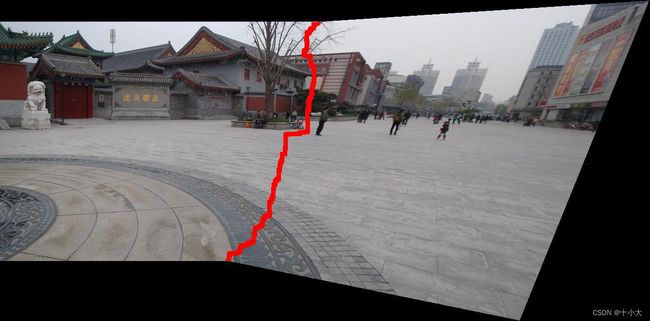
可视化：

        % 可视化迭代过程
        final_out = gradientBlend(warped_img1, final_As, warped_img2);
        final_Bs = (A|B) & ~final_As;
        C_seam = imdilate(final_As, square_SE) & imdilate(final_Bs, square_SE) & C;
        final_seam = final_out;
        final_seam(cat(3, C_seam, C_seam, C_seam)) = [ones(sum(C_seam(:)),1); zeros(2*sum(C_seam(:)),1)];
        fprintf('final output comes from k_seam = %d\n', k_seam-1);
        figure,imshow(final_out);
        figure,imshow(final_seam);
        %outpath = sprintf('%d-final_out.jpg',k_seam-1)
        %imwrite(final_out, outpath)
        %outpath1 = sprintf('%d-final_seam.jpg',k_seam-1)
        %imwrite(final_seam, outpath1)

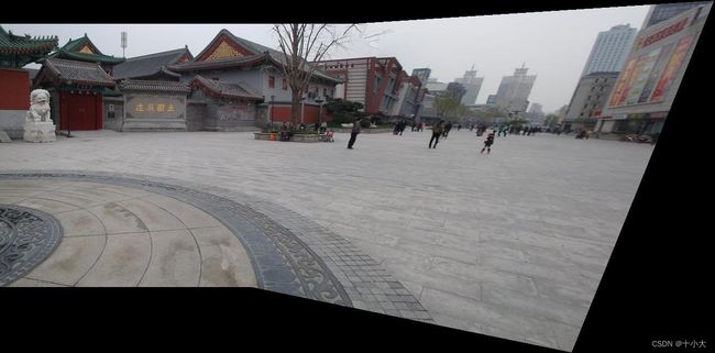
如果将可视化部分的代码段写在循环内，则可以观察到接缝变化的过程。这里我们用temple数据集试着展示图3中的接缝变化过程，用红色表示接缝。

( a ) Initial iteration:

( b ) Middle iteration:

( c ) Latter iteration:

( d ) Final result:

至此，本文的代码已解读完毕。

3. 总结思考，试图创新

还是回到论文中的创新点：

1. 迭代接缝估计算法，校正错位的接缝
2. 质量评估算法能得到错位的地方，能为后续的接缝方法提供接缝评估手段
   PS：已经在后文Seam-guided local alignment and stitching for large parallax images中做到了。

重温一下算法1和算法2加深印象：

算法1：

1. 对每个接缝上的像素，计算像素点成本和块成本
2. 得到上面两个的信号值
3. 小波去噪平滑信号，得到两个去噪后的成本
4. 计算去噪后的混合成本
   
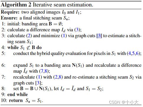
   算法2：
5. 初始化区域（两边各扩展5像素）
6. 计算差异图
7. 图割计算接缝
8. 不满足条件时
9. 扩展像素、重新计算差异图、图割得到新的接缝，重复这三步，直到跳出循环

拼接结果对比展示：

初始接缝拼接结果：

本文算法的结果：

可以看到，初始的接缝破坏了原有的结构（树），而本文的算法经过迭代优化接缝，得到了比较不错的效果。

本文的创新已在【图像拼接】源码精读：Seam-guided local alignment and stitching for large parallax images中实现。

感谢同学们阅读本文，如果对你有所帮助，点个赞，点个收藏吧，我们下一篇论文源码精读再会！