【图像拼接】源码精读:Seam-guided local alignment and stitching for large parallax images
第一次来请先看这篇文章:【图像拼接(Image Stitching)】关于【图像拼接论文源码精读】专栏的相关说明,包含专栏内文章结构说明、源码阅读顺序、培养代码能力、如何创新等(不定期更新)
【图像拼接论文源码精读】专栏文章目录
- 【源码精读】As-Projective-As-Possible Image Stitching with Moving DLT(APAP)第一部分:全局单应Global homography
文章目录
- 【图像拼接论文源码精读】专栏文章目录
- 前言
- 1. 跑通代码,得到结果
-
- 1.1 准备工作
- 1.2 尝试运行
- 1.3 得到拼接结果
- 2. 源码解读,看懂原理
-
- 2.1 参数与输入图像
- 2.2 图像对齐
-
- 2.2.1 总体流程
- 2.2.2 siftMatch函数
- 2.2.3 homoRANSAC函数
- 2.2.4 calcHomo函数
- 2.2.5 homographyAlign函数
- 2.2.6 小结
- 2.3 接缝融合,blendTexture函数
-
- 2.3.1 找重叠区域边界,并得到基于感知的接缝切割算法的【数据项】
- 2.3.2 可视化重叠区域边界(新增代码)
- 2.3.3 基于感知的接缝切割算法的【平滑项】
- 2.3.4 图割+梯度融合得到拼接结果
- 2.3.5 可视化拼接结果(带接缝)
- 2.3.6 沿着接缝找没对齐的地方,进行修补(论文算法核心,代码对应论文中3.2和3.3部分)
- 2.3.7 (论文算法核心,代码对应论文中3.4和3.5部分)
- 3. 总结思考,试图创新
前言
论文题目:Seam-guided local alignment and stitching for large parallax images——大视差图像的接缝引导局部对齐和拼接
论文地址:Seam-guided local alignment and stitching for large parallax images
论文源码:https://github.com/tlliao/Seam-guided-local-alignment
注:matlab源码,相关算法是C++封装的。主要是对matlab的学习与理解。

论文精读:【图像拼接】论文精读:Seam-guided local alignment and stitching for large parallax images
配合【论文精读】专栏对应文章阅读,效果更佳!
注:请重点关注代码段中的注释!!!有一些讲解的东西直接写在代码段的注释中了,同时多关注红色字体和绿色字体!!!
1. 跑通代码,得到结果
任何源码下载下来后,第一件事就是先跑通。
无论你是否要在该工作的基础上创新,总是需要得到拼接结果,在论文的实验部分做对比。
所以,请务必跑通,得到拼接结果。
1.1 准备工作
本地需要matlab环境,我是MATLAB R2018b,选择一个适中的matlab版本即可。(最新的matlab2023可以使用局部函数了,类似jupyter notebook,感兴趣的同学可以试试最新版。)
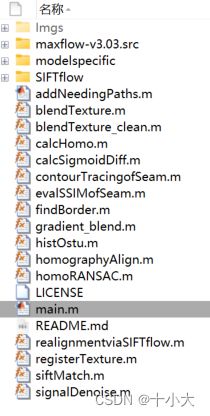
源码下载下来后,用matlab打开项目,界面如下:
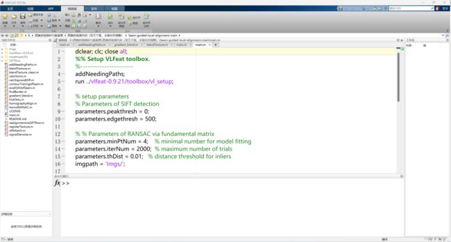
左侧是文件目录结构,中级是当前所选文件代码,下面是命令行窗口,右侧是工作区(运行后显示相关变量的值)
1.2 尝试运行
点击上面菜单栏【运行】,出现如下报错:

检查后发现,当前目录下没有vlfeat-0.9.21文件夹:
我们在其他论文的源码中将vlfeat-0.9.21文件夹整个复制到该目录下即可:

并将报错位置的代码修改为:
% run ../vlfeat-0.9.21/toolbox/vl_setup;
run vlfeat-0.9.21/toolbox/vl_setup;
再次运行后:

代码已经可以完整的跑通了。
1.3 得到拼接结果
我们发现,源码并没有显示拼接结果。在main.m中末尾添加显示结果:
f = figure;
imshow(seam_cut,'border','tight');
hold on;
再次运行后,得到1_l.jpg和1_r.jpg的拼接结果:
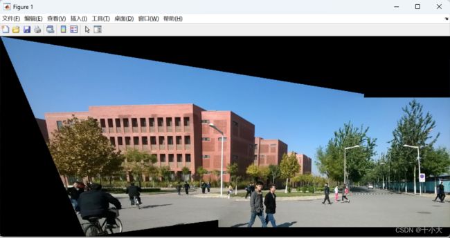
原图为:
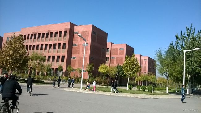 1_l.jpg 1_l.jpg
|
 1_r.jpg 1_r.jpg
|
附上原作者README中的使用方法:

2. 源码解读,看懂原理
本节将按照main.m中的代码顺序进行【模块化】讲解,包括与论文中的算法对应、matlab语法和函数学习、变量的类型和值、函数功能等方面。代码段中包含原作者的注释和我做的注释,与讲解结合着阅读。
2.1 参数与输入图像
代码如下:
%% Setup VLFeat toolbox.
%----------------------
addNeedingPaths;
% 刚下载下来的源码,没有vlfeat-0.9.21文件夹
% run ../vlfeat-0.9.21/toolbox/vl_setup;
run vlfeat-0.9.21/toolbox/vl_setup;

% setup parameters
% Parameters of SIFT detection
parameters.peakthresh = 0;
parameters.edgethresh = 500;

% % Parameters of RANSAC via fundamental matrix
parameters.minPtNum = 4;    % minimal number for model fitting
parameters.iterNum = 2000;  % maximum number of trials
parameters.thDist = 0.01;   % distance threshold for inliers

imgpath = 'Imgs/';
img_format = '4_*.jpg'; % 以论文中图1为例
dir_folder = dir(strcat(imgpath, img_format)); %连接路径,列出文件夹中的内容

path1 =  sprintf('%s%s',imgpath, dir_folder(1).name); % 路径转换成字符串
path2 =  sprintf('%s%s',imgpath, dir_folder(2).name); %
img1 = im2double(imread(path1));  % target image         图像转成双精度,后面SIFT的输入要求是双精度
img2 = im2double(imread(path2));  % reference image
主要包含SIFT算法参数、RANSAC算法参数、输入两张图像的路径、得到双精度的目标图和参照图。
2.2 图像对齐
代码如下:
%% image alignment
fprintf('> image alignment...');
tic; % 计时器
[pts1, pts2] = siftMatch(img1, img2, parameters);
[matches_1, matches_2] = homoRANSAC(pts1, pts2, parameters);
init_H=calcHomo(matches_1, matches_2);
[warped_img1, warped_img2] = homographyAlign(img1, img2, init_H);
fprintf('done (%fs)\n', toc);   % 输出时间
2.2.1 总体流程
- 对两张输入图像应用SIFT算法,得到两张图像的特征点pts1,pts2;
- 通过RANSAC算法得到两张图像的匹配点,即内点(inliers)matches_1,matcher_2;
- 通过匹配点得到初始的单应矩阵init_H;
- 根据单应矩阵init_H得到翘曲后的两张图像warped_img1,warped_img2;
接下来我们具体解读上述步骤中的函数。
2.2.2 siftMatch函数
函数功能:得到两张图的特征点,输入两张图像和算法参数,返回值为两张图像的特征点。
对应根目录下文件siftMatch.m,代码如下:
function [pts1, pts2] = siftMatch( img1, img2, parameters )
%--------------------------------------
% SIFT keypoint detection and matching.
%--------------------------------------
peakthresh = parameters.peakthresh;
edgethresh = parameters.edgethresh;
%fprintf('  Keypoint detection and matching...');tic;
[ kp1,ds1 ] = vl_sift(single(rgb2gray(img1)),'PeakThresh', peakthresh,'edgethresh', edgethresh);
[ kp2,ds2 ] = vl_sift(single(rgb2gray(img2)),'PeakThresh', peakthresh,'edgethresh', edgethresh);
matches   = vl_ubcmatch(ds1, ds2);
%fprintf('done (%fs)\n',toc);

% extract match points' position
pts1 = kp1(1:2,matches(1,:));
pts2 = kp2(1:2,matches(2,:));

end
前文【源码精读】As-Projective-As-Possible Image Stitching with Moving DLT(APAP)第一部分:全局单应Global homography已经讲过,包括每个函数、每个变量的含义,非常详细。本节不再赘述。
2.2.3 homoRANSAC函数
函数功能:使用MATLAB自带的RANSAC函数,去除特征匹配点中的异常值,得到内点索引,进而得到所有的正常匹配点。
对应根目录下文件homoRANSAC.m,代码如下:
function [matches_1, matches_2] = homoRANSAC(pts1, pts2, parameters)
% using fundamental matrix for robust fitting

minPtNum = parameters.minPtNum;  % minimal number of points to estimate H and e
iterNum = parameters.iterNum;  % maximum iterations
thDist = parameters.thDist;  % distance threshold
% ptNum = size(pts1, 2);  % number of points

%% perform coordinate normalization
[normalized_pts1, ~] = normalise2dpts([pts1; ones(1,size(pts1, 2))]);
[normalized_pts2, ~] = normalise2dpts([pts2; ones(1,size(pts2, 2))]);
points = [normalized_pts1', normalized_pts2']; % n×6 [x1 y1 1 x2 y2 1]

% @(points):这部分定义了一个匿名函数,在 MATLAB 中使用 @ 符号表示创建一个函数。
% 括号中的 points 是函数的输入参数,表示这个函数接受一个名为 points 的参数。
% 这么写是为了适配下面的ransac函数的输入,必须是function_handle
fitmodelFcn = @(points)calcNormHomo(points); % fit function,拟合函数 9×1
evalmodelFcn = @(homo, points)calcDistofHomo(homo, points); % 距离 1×n

rng(0); % 设置随机种子,让每次重启程序的RANSAC一致
% matlab自带的ransac算法,其实我觉得用APAP那一套RANSAC更方便一些
[~, inlierIdx] = ransac(points,fitmodelFcn,evalmodelFcn,minPtNum,thDist,'MaxNumTrials',iterNum);

inliers1 = pts1(:, inlierIdx);
inliers2 = pts2(:, inlierIdx);

matches_1 = inliers1;
matches_2 = inliers2;

% delete duplicate feature match
[~,  ind1] = unique(matches_1', 'rows');
[~,  ind2] = unique(matches_2', 'rows');
ind = intersect(ind1, ind2);
matches_1 = matches_1(:, ind);
matches_2 = matches_2(:, ind);

end

function [ homo ] = calcNormHomo(points) % estimate H_inf and e' via DLT
% 求解单应矩阵的过程,先随便计算一个矩阵H',得到模型。RANSAC第一步

npts1 = points(:, 1:3)';
npts2 = points(:, 4:6)';

%% calculation the initial H0 and e0
Equation_matrix = zeros(2*size(npts1, 2), 9);
for i=1:size(npts1, 2)
    xi = npts1(1,i); yi = npts1(2,i);
    xi_= npts2(1,i); yi_= npts2(2,i);
    tmp_coeff1 = [xi, yi, 1, 0,  0,  0, -xi*xi_, -yi*xi_, -xi_];
    tmp_coeff2 = [0,  0,  0, xi, yi, 1, -xi*yi_, -yi*yi_, -yi_];
    Equation_matrix(2*i-1:2*i, :) = [tmp_coeff1; tmp_coeff2];
end

[~,~,v] = svd(Equation_matrix, 0);
norm_homo = reshape(v(1:9, end), 3, 3)';
homo = norm_homo(:);    % 按列排序,排成1列

end

function dist = calcDistofHomo(homo, points) % calculate the projective error
% 计算投影误差,看手写部分,RANSAC第二步
% RANSAC最后一步就是用自带的ransac函数迭代,找比这个误差小的作为内点,更新H',返回模型和索引

pts1 = points(:, 1:3)';
pts2 = points(:, 4:6)';

H = reshape(homo(1:9),3,3); % 和上面norm_homo一样

tmp1 = (H(1,:)*pts1)./pts1(3,:);
tmp2 = (H(2,:)*pts1)./pts1(3,:);
tmp3 = (H(3,:)*pts1)./pts1(3,:);
mapped_pts2(1,:) = tmp1./tmp3;
mapped_pts2(2,:) = tmp2./tmp3;
dist = sqrt(sum((mapped_pts2-pts2(1:2,:)).^2, 1));

end
RANSAC过程以及代码对应:
- 随机抽出m(m>4)个样本数据,计算出单应性矩阵H’,记为模型M;
- 使用剩余的点对计算投影误差,检测误差小于设置阈值的点的个数,如果个数多于之前记录的最优值,则替换H’,并记录此次的点数为最优值;
- 是否达到设置的迭代次数,若是,则输出H’并结束,否则重新迭代,回到步骤1;
步骤1对应calcNormHomo函数,步骤2对应calcDistofHomo函数,步骤3对应homoRANSAC中的ransac函数。
其中,calcNormHomo函数是计算单应矩阵的过程,详解见【源码精读】As-Projective-As-Possible Image Stitching with Moving DLT(APAP)第一部分:全局单应Global homography。有手写的公式推导。
重点讲一下投影误差计算calcDistofHomo函数。
计算出H’(对应函数中的H)后,使用如下公式进行投影误差计算:
E p r o j = ∑ i = 0 n ( ( x i ′ − h 11 x i + h 12 y i + h 13 h 31 x i + h 32 y i + h 33 ) 2 + ( y i ′ − h 21 x i + h 22 y i + h 23 h 31 x i + h 32 y i + h 33 ) 2 ) E_{proj} = \sqrt{\sum_{i =0}^n((x_i' - \frac{h_{11}x_i+h_{12}y_i+h_{13}}{h_{31}x_i+h_{32}y_i+h_{33}})^2+(y_i' - \frac{h_{21}x_i+h_{22}y_i+h_{23}}{h_{31}x_i+h_{32}y_i+h_{33}})^2)} Eproj=i=0∑n((xi′−h31xi+h32yi+h33h11xi+h12yi+h13)2+(yi′−h31xi+h32yi+h33h21xi+h22yi+h23)2)
代码中的tmp1为 h 11 x i + h 12 y i + h 13 h_{11}x_i+h_{12}y_i+h_{13} h11xi+h12yi+h13,tmp2为 h 21 x i + h 22 y i + h 23 h_{21}x_i+h_{22}y_i+h_{23} h21xi+h22yi+h23,tpm3为 h 31 x i + h 32 y i + h 33 h_{31}x_i+h_{32}y_i+h_{33} h31xi+h32yi+h33。过程就是计算上面的公式,得到投影误差。
最后,经过matlab自带的ransac函数得到正常匹配点索引,进而得到匹配点。
2.2.4 calcHomo函数
函数功能:计算DLT(直接线性变换)得到全局单应矩阵。
对应根目录下文件calcHomo.m,代码如下:
function H = calcHomo(pts1,pts2)
%% use Direct linear tranformation (DLT) to calculate homography
%  approxmation: H*[pts1; ones(1,size(pts1,2))] = [pts2; ones(1,size(pts2,2))]
% Normalise point distribution.
data_pts = [ pts1; ones(1,size(pts1,2)) ; pts2; ones(1,size(pts2,2)) ];
[ dat_norm_pts1,T1 ] = normalise2dpts(data_pts(1:3,:));
[ dat_norm_pts2,T2 ] = normalise2dpts(data_pts(4:6,:));
data_norm = [ dat_norm_pts1 ; dat_norm_pts2 ]; % 6×n,同APAP中全局单应部分

%-----------------------
% Global homography (H).
%-----------------------
%fprintf('DLT (projective transform) on inliers\n');
% Refine homography using DLT on inliers.
%fprintf('> Refining homography (H) using DLT...');
[ h,~,~,~ ] = homography_fit(data_norm);    % 计算DLT,得到9×1
H = T2\(reshape(h,3,3)*T1); % 得到初始的全局单应矩阵

end
其中,homography_fit函数为:
function [P A C1 C2] = homography_fit(X,A,W,C1,C2)
% 得到9×1的单应矩阵P
x1 = X(1:3,:);  % 两个图的点,3×n,[x y 1]
x2 = X(4:6,:);

if nargin == 5
    H = vgg_H_from_x_lin(x1,x2,A,W,C1,C2);
else
    [H A C1 C2] = vgg_H_from_x_lin(x1,x2);  % 只传一个参数会进入这里
end

P = H(:);   % 9 ×1

end
再进一步,vgg_H_from_x_lin函数为:
function [H, A, C1, C2] = x(xs1,xs2,A,W,C1,C2)
    % 函数功能:计算DLT
    % 返回值含义:
    % H:3×3单应矩阵,h33为1
    % A:Ah = 0 的A,最小二乘计算先新变化
    % C1、C2:归一化矩阵

    % H = vgg_H_from_x_lin(xs1,xs2)
    %
    % Compute H using linear method (see Hartley & Zisserman Alg 3.2 page 92 in
    %                              1st edition, Alg 4.2 page 109 in 2nd edition).
    % Point preconditioning is inside the function.
    %
    % The format of the xs [p1 p2 p3 ... pn], where each p is a 2 or 3
    % element column vector.

    [r,c] = size(xs1); % r是行数,此处使用为3;c是点的个数

    if (size(xs1) ~= size(xs2)) % 如果两个匹配点数量不同,报错
     error ('Input point sets are different sizes!')
    end

    if (size(xs1,1) == 2)   % 如果是非齐次的,则齐次化
      xs1 = [xs1 ; ones(1,size(xs1,2))];
      xs2 = [xs2 ; ones(1,size(xs2,2))];
    end


    % condition points,只传了两组特征点坐标进入这里
    if nargin == 2
        C1 = vgg_conditioner_from_pts(xs1); % 两个点集的调节矩阵
        C2 = vgg_conditioner_from_pts(xs2);
        xs1 = vgg_condition_2d(xs1,C1);        % 得到归一化后的坐标
        xs2 = vgg_condition_2d(xs2,C2);
    end

    if nargin == 6
        B = A;
        B(1:2:end,:)=W*A(1:2:end,:);
        B(2:2:end,:)=W*A(2:2:end,:);

        % Extract nullspace
        [u,s,v] = svd(B, 0); s = diag(s);
    else
        A = [];
        ooo  = zeros(1,3);
        for k=1:c % 取每个点
          p1 = xs1(:,k);    % 得到齐次坐标
          p2 = xs2(:,k);
          A = [ A;
            p1'*p2(3) ooo -p1'*p2(1)
            ooo p1'*p2(3) -p1'*p2(2)
           ];   % 得到2n × 9,Ah=0 的A: [ x y 1 0 0 0 -xx' -yx' -x']
                %                       [ 0 0 0 x y 1 -xy' -yy' -y']
                % 反正是解方程,等式右边是0矩阵,-A和A一样
        end

        % Extract nullspace
        [u,s,v] = svd(A, 0); %svd分解
        s = diag(s);
    end

    nullspace_dimension = sum(s < eps * s(1) * 1e3);
    if nullspace_dimension > 1
      fprintf('Nullspace is a bit roomy...');
    end

    h = v(:,9); %要v的最右列向量,9×1

    H = reshape(h,3,3)'; % 变成 3×3

    %decondition
    H = C2\H*C1;    % 调节回去,去归一化

    H = H/H(3,3);   % h33变成1
end
vgg_condition_2d函数:
function pc = z(p,C)
% 函数功能:使用调节矩阵,调节点集,得到归一化后的坐标点
% function pc = vgg_condition_2d(p,C);
%
% Condition a set of 2D homogeneous or nonhomogeneous points using conditioner C

[r,c] = size(p);
if r == 2
  pc = vgg_get_nonhomg(C * vgg_get_homg(p));
elseif r == 3
  pc = C * p;   % 3维点,每个点左乘调节矩阵
else
  error ('rows != 2 or 3');
end

end
上面函数跟着阅读注释即可。重点理解vgg_H_from_x_lin函数,在文件夹modespecific中,都是一些通用方法。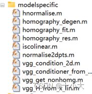
2.2.5 homographyAlign函数
函数功能:得到参照图和目标图翘曲后的图像
对应根目录下文件homographyAlign.m,代码如下:
function [ homo1, homo2] = homographyAlign( img1,img2,init_H )
%input: target image and reference image, saliency map of the two images
%output: homography-warped target and reference, with their corresponding
%saliency maps
tform = projective2d(init_H');  % 根据全局单应得到2d投影对象,与imwarp同时使用
img1mask = imwarp(true(size(img1,1),size(img1,2)), tform, 'nearest');   % 得到img1的掩码

img1To2 = imwarp(img1, tform);  % 得到变换后的图像
img1To2 = cat(3,img1mask, img1mask, img1mask).*img1To2; % 用掩码再处理一下
%注:可视化上面两个目标图,几乎没有区别,用掩码在三个通道分别处理一下,可能是为了修正图像

pt = [1, 1, size(img1,2), size(img1,2);
      1, size(img1,1), 1, size(img1,1);
      1, 1, 1, 1];  % 图像四个角点列向量
H_pt = init_H*pt; % 得到变换后的点
H_pt = H_pt(1:2,:)./repmat(H_pt(3,:),2,1);  %归一化,齐次转非齐次

% calculate the convas
% 计算画布大小,适配两张图像
off = ceil([ 1 - min([1 H_pt(1,:)]) + 1 ; 1 - min([1 H_pt(2,:)]) + 1 ]);
cw = max(size(img1To2,2)+max(1,floor(min(H_pt(1,:))))-1, size(img2,2)+off(1)-1);
ch = max(size(img1To2,1)+max(1,floor(min(H_pt(2,:))))-1, size(img2,1)+off(2)-1);

% 目标图翘曲后的画布肯定能容纳下参照图,所以就用目标图的画布大小
homo1 = zeros(ch,cw,3); homo2 = zeros(ch,cw,3); %

% 填充两张图像到画布中
homo1(floor(min(H_pt(2,:)))+off(2)-1:floor(min(H_pt(2,:)))+off(2)-2+size(img1To2,1),...
    floor(min(H_pt(1,:)))+off(1)-1:floor(min(H_pt(1,:)))+off(1)-2+size(img1To2,2),:) = img1To2;
homo2(off(2):(off(2)+size(img2,1)-1),off(1):(off(1)+size(img2,2)-1),:) = img2;

end
注:计算画布那里原作者的注释写错了,是canvas不是convas。
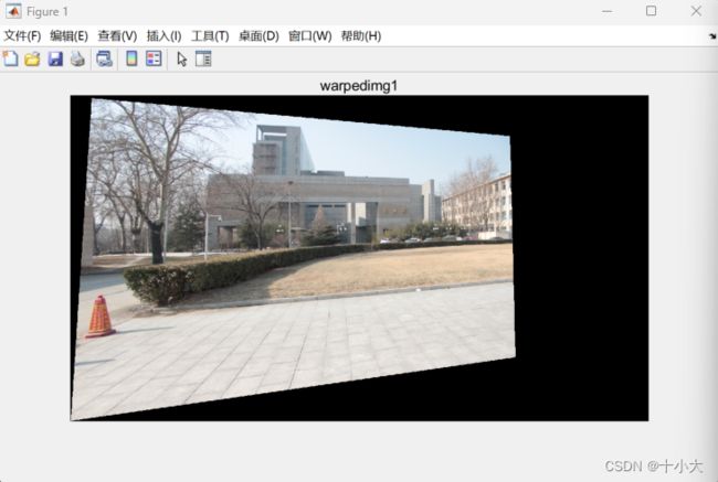
在主函数中添加可视化代码:
figure;
imshow(warped_img1);
title('warpedimg1');
figure;
imshow(warped_img2);
title('warpedimg2');

% 平均融合,除2非重叠区域暗,重叠区域原亮度;不除2则是非重叠区域原亮度,重叠区域更亮
% 原论文图1(b)的是TFA得到的,而不是此处的单应变换
output_canvas(:,:,1) = (warped_img1(:,:,1)+warped_img2(:,:,1))/2;
output_canvas(:,:,2) = (warped_img1(:,:,2)+warped_img2(:,:,2))/2;
output_canvas(:,:,3) = (warped_img1(:,:,3)+warped_img2(:,:,3))/2;

figure;
imshow(output_canvas);
title('output_canvas');
翘曲后的两张图像和拼接结果如下,使用论文图1中的数据:

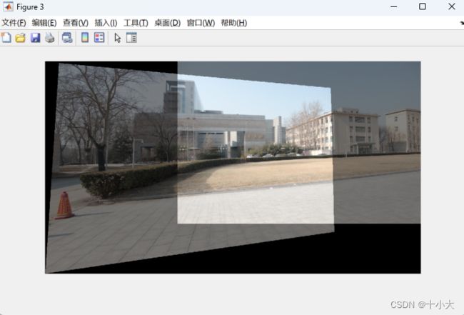
2.2.6 小结
本节详细讲解了两张图像对齐的流程,首先通过SIFT得到特征点,然后经过RANSAC筛选,得到正常匹配点,最后将参照图和目标图翘曲。添加了可视化代码,得到拼接结果,实现了论文中图1的,重叠区域保持原亮度,非重叠区域暗一些的效果。
读代码的方法: 1. 紧跟变量流,包括特征点流、图像流等 2. 把函数单拿出来测试,matlab的工作区可以显示变量的结构和值 比如:SIFT和RANSAC的部分,就是特征点流,一系列的处理都是围绕特征匹配点展开的,重点关注特征点的向量如何变化,包括特征点的结构、取值、行列变换、齐次化等。前面都是一些铺垫和准备工作,是其他论文中已经实现的预对齐步骤。下一节是本论文的核心部分,我将重点讲解,并与论文中的部分对应。
2.3 接缝融合,blendTexture函数
2.3.1和2.3.3对应论文的3.1部分Conventional Seam-cutting和算法1中的步骤1,是Perception-based-seam-cutting论文中基于感知的接缝算法得到的初始接缝,通过数据项和平滑项,经过图割和梯度融合得到拼接结果。
2.3.6对应论文的3.2 SSIM-based Seam Evaluation和3.3 Components Extraction部分,算法1中步骤2,3,4,5。SSIM误差是论文Quality evaluation-based iterative seam estimation for image stitching中提出的,根据SSIM误差和Ostu算法得到的阈值比较,得到未对齐的接缝像素点和块。
2.3.7对应论文的3.4 Patch Alignment和3.5 Seam Merging部分,算法1中步骤6,7,8,9,10,11,12。将未对齐的块分离开,使用SIFTflow算法获得流向量,用公式(4)中的sigmoid函数修正流向量,进而对齐块,计算新的接缝,用新的接缝(块)替换原图中的接缝(块)。
代码如下:
%% image composition
fprintf('> seam cutting...');tic;
[seam_cut] = blendTexture(warped_img1, warped_img2);
fprintf('done (%fs)\n', toc);
本节我们将一段一段讲解blendTexture.m文件下对应的代码,也是本论文的核心。
2.3.1 找重叠区域边界,并得到基于感知的接缝切割算法的【数据项】
seam-cutting预处理:
%%  pre-process of seam-cutting
w1 = imfill(imbinarize(rgb2gray(warped_img1), 0),'holes'); % 翘曲图灰度化、二值化、黑色变白色
w2 = imfill(imbinarize(rgb2gray(warped_img2), 0),'holes');
A = w1;  B = w2;
C = A & B;  % mask of overlapping region,重叠区域像素值为1,其余为0
[ sz1, sz2 ]=size(C);
ind = find(C);  % index of overlapping region,重叠区域索引
nNodes = size(ind,1);   % 重叠区域像素个数
revindC = zeros(sz1*sz2,1); % 反向索引,初始全是0,整张图
revindC(C) = 1:length(ind); % 重叠区域中的索引顺序
得到重叠区域边界以及数据项作为图割算法输入参数:
%%  terminalWeights, choose source and sink nodes
% 这段代码是在找重叠区域边界

border_B = findBorder(B);   %参照图边界
border_C = findBorder(C);   %重叠区域边界

imgseedA = border_B & border_C; % 参照图与重叠区域相交的两条边
imgseedB = ~imgseedA & border_C;   % 目标图翘曲后与重叠区域相交的两条边

% data term
tw=zeros(nNodes,2); % 初始化数据项权重
tw(revindC(imgseedA),1)=inf;    % 第一列(对应于标签1)的权重设置为正无穷
tw(revindC(imgseedB),2)=inf;    % 第二列(对应于标签2)的权重设置为正无穷

terminalWeights=tw;       % data term,得到图割算法中的数据项

% 上面代码的目的是为了图割算法中,通过最小化数据项权重来实现图割算法,将边界设置为无穷大方便后续计算。
其中,找边界用的是错位差分法。对应的函数文件为findBorder.m:
function [ border_img ] = findBorder( mask_img )
% give a mask image, find its border, (boundary points)
% border of mask image
[sz1, sz2] = size(mask_img);
mask_R=(mask_img-[mask_img(:,2:end) false(sz1,1)])>0;   %右边界
mask_L=(mask_img-[false(sz1,1) mask_img(:,1:end-1)])>0; %左边界
mask_D=(mask_img-[mask_img(2:end,:);false(1,sz2)])>0;   % 下边界
mask_U=(mask_img-[false(1,sz2);mask_img(1:end-1,:)])>0; %上边界
border_img = mask_R | mask_L | mask_D | mask_U;

% 差分操作,列方向往右平移一个像素,然后通过差分判断是否大于0,从而得到边界
% 最后合并边界信息,边界像素值为1,其他地方为0
end
2.3.2 可视化重叠区域边界(新增代码)
我们添加可视化代码,显示重叠区域边界:
%% 可视化重叠区域边界

[m,~] = find(C);    % 找最大最小行
minrow = min(m);
maxrow = max(m);

mask=~(imgseedB | imgseedA); %掩码 重叠区域边界为0
% 将两个翘曲图像对齐并添加权重,跟前面显示图像拼接结果一样,0.5是平均融合,亮度与原图一致
imglap = 0.5.*imadd(warped_img1.*cat(3,mask&C,mask&C,mask&C), warped_img2.*cat(3,mask&C,mask&C,mask&C));

% free_seed中没有最小最大行索引对应的行
freeseed = imgseedA;
freeseed(minrow,:) = 0;
freeseed(maxrow,:) = 0;
free_seed = imgseedA & (~freeseed);

% 种子区域权重设置为0
tw(revindC(free_seed),1) = 0;
tw(revindC(free_seed),2) = 0;
imgseed = warped_img1.*cat(3,A-C,A-C,A-C) + warped_img2.*cat(3,B-C,B-C,B-C) + imglap+cat(3,freeseed,free_seed,imgseedB);
% imgseed = warped_img1.*cat(3,A-C,A-C,A-C) + warped_img2.*cat(3,B-C,B-C,B-C)+ imglap

% cat(3,A-C,A-C,A-C):目标图重叠区域边界为红色(R通道高亮)
% cat(3, B - C, B - C, B - C):参照图重叠区域边界标记为蓝色(B通道高亮)
% cat(3,freeseed,free_seed,imgseedB): 会影响部分边界颜色变为绿色(G通道高亮),不加这一项边界都是黑色
% 三色组合显示重叠区域边界

% 可视化
figure,imshow(imgseed);
title('seed image on two warped images');

% 如果要保存的话
% pngout = sprintf('Overlapping_result.png');
% imwrite(imgseed,pngout);
可视化结果:
注:这里代码与Perception-based-seam-cutting中的类似,将找边界封装成函数了。
2.3.3 基于感知的接缝切割算法的【平滑项】
计算平滑项:
%% calculate edgeWeights
% 四个边界为0的掩码
CL1=C&[C(:,2:end) false(sz1,1)];   % 与C比,最右一列为0
CL2=[false(sz1,1) CL1(:,1:end-1)];  % 最左一列为0
CU1=C&[C(2:end,:);false(1,sz2)];    % 最下一行
CU2=[false(1,sz2);CU1(1:end-1,:)];  % 最上一行

%  edgeWeights:  sigmoid-metric difference map,sigmoid差异图
[imgdif_sig, ~] = calcSigmoidDiff(warped_img1, warped_img2, C);

% sigmoid method,用于衡量图像中相邻区域的差异,即图像变化的平滑度
DL = (imgdif_sig(CL1)+imgdif_sig(CL2))./2;  % 水平方向上平均值
DU = (imgdif_sig(CU1)+imgdif_sig(CU2))./2;  % 垂直方向上平均值

% smoothness term
edgeWeights=[
    revindC(CL1) revindC(CL2) DL+1e-8 DL+1e-8;
    revindC(CU1) revindC(CU2) DU+1e-8 DU+1e-8];

% 每一行一个边界,包含各边界索引和对应的平滑项值,小偏移量1e-8,防止分母为0
通过sigmoid函数计算差异,calcSigmoidDiff.m:
unction [ imgdif_sig, imgdif ] = calcSigmoidDiff(img1, img2, C)
% 函数功能:计算两张图像差异,返回一个sigmoid函数差异图

%  edgeWeights:  Euclidean-weighted norm
% 两张图像三通道分量
ang_1=img1(:,:,1); sat_1=img1(:,:,2); val_1=img1(:,:,3);
ang_2=img2(:,:,1); sat_2=img2(:,:,2); val_2=img2(:,:,3);

% baseline difference map,两个图像每个像素位置上RGB通道的差异
imgdif = sqrt( ( (ang_1.*C-ang_2.*C).^2 + (sat_1.*C-sat_2.*C).^2 + (val_1.*C-val_2.*C).^2 )./3 );

% sigmoid-metric difference map
a_rgb = 0.06; % bin of histogram
beta=4/a_rgb; % beta
gamma=exp(1); % base number
para_alpha = histOstu(imgdif(C), a_rgb);  % parameter:tau
imgdif_sig = 1./(1+power(gamma,beta*(-imgdif+para_alpha))); % difference map with logistic function
imgdif_sig = imgdif_sig.*C;   % difference to compute the smoothness term

% 使用 Sigmoid 函数将 imgdif 映射到 (0, 1) 范围内,得到 imgdif_sig。
% 然后,通过与掩码 C 相乘,仅保留 C 中为真的区域的值,这样可以计算平滑项(smoothness term)。
% 对应论文中计算平滑项的公式

end
上面数据项与平滑项的理论来自于文章Perception-based energy functions in seam-cutting。对应的论文精读为:
2.3.4 图割+梯度融合得到拼接结果
图割得到接缝的标签矩阵,值为1是接缝的像素,然后梯度融合得到拼接结果:
%%  graph-cut labeling
[~, labels] = graphCutMex(terminalWeights, edgeWeights);

As=A;
Bs=B;
As(ind(labels==1))=false;   % mask of target seam
Bs(ind(labels==0))=false;   % mask of reference seam
imgout = gradient_blend(warped_img1, As, warped_img2);

SE_seam = strel('diamond', 1);
As_seam = imdilate(As, SE_seam) & A;
Cs_seam = As_seam & Bs;	% 重叠区域最终的接缝,像素值为1,其余为0
2.3.5 可视化拼接结果(带接缝)
我们添加可视化代码,显示拼接缝:
%% 可视化接缝
imgseam = imgout.*cat(3,(A|B)-Cs_seam,(A|B)-Cs_seam,(A|B)-Cs_seam) + cat(3,Cs_seam,zeros(sz1,sz2),zeros(sz1,sz2));

figure,imshow(imgseam);
title('final stitching seam');
SE_seam中的strel第二个参数条件接缝粗细。
2.3.6 沿着接缝找没对齐的地方,进行修补(论文算法核心,代码对应论文中3.2和3.3部分)
- 找到接缝上所有像素点的坐标
- 给接缝上所有像素点定义一个20×20的块,每个块计算SSIM误差
- 如果所得的SSIM误差最大值都在范围内,则是合理的接缝
- 否则,根据Ostu算法得到阈值tou,找到接缝上比该阈值大的块和像素点
该模块代码如下:
%%  find potential artifacts along the seam for patch mark
% 沿着拼接缝找没对齐的地方,然后修补

% extract pixels on the seam and evaluate the patch error
% 提取接缝处的像素,并评估补丁误差

seam_pts = contourTracingofSeam(Cs_seam);   % 接缝上所有点的坐标[行,列],是整张图的索引
[ssim_error, ~, patch_coor] = evalSSIMofSeam(warped_img1, warped_img2, C, seam_pts, patch_size);    %每个像素点的SSIM误差和块范围

% 对应论文3.3部分
% mark misaligned local regions
% max(Q) <= kmean(Q)
if max(ssim_error)<=1.5*mean(ssim_error)    % 接缝所有的像素点都在误差允许范围内,则接缝合理,直接就是结果
    seam_cut=imgout;
    return;
end

T = graythresh(ssim_error); % Ostu的阈值tou, 以图4为例,T=0.1882
artifacts_pixels = seam_pts(ssim_error>=T,:);   % 找到所有比阈值大的像素坐标
artifacts_patchs = patch_coor(ssim_error>=T,:); % 比阈值大的块的范围

% 错位像素、和错位像素的块的掩码
artifacts_masks = false(sz1,sz2);
mask_pixels = false(sz1,sz2);
for i=1:size(artifacts_patchs,1)
    artifacts_masks(artifacts_patchs(i,1):artifacts_patchs(i,2),artifacts_patchs(i,3):artifacts_patchs(i,4))=1;
    mask_pixels(artifacts_pixels(i,1),artifacts_pixels(i,2))=1;
end

% add modification to artifacts_masks: connect neighboring patches if they
% are close enough
% 如果相邻的块足够近,则连上
artifacts_masks = imclose(artifacts_masks, strel("square",10));
找到接缝上所有像素点的坐标,contourTracingofSeam.m:
function [ BoundaryPts ] = contourTracingofSeam( mask_seam )
% tracing the image seam of the stitched image
% B_seam: binary image with only seam mask
% BoundaryPts: contour coordinates [rows, cols]
% the contour points are in white region

% 函数功能:拼接图的接缝轮廓跟踪
% 输入mask_seam:逻辑二值接缝
% 返回值BoundaryPts:论文坐标[行,列]
    Movement = [0, 1;
                1, 1;
                1, 0;
                1,-1;
                0,-1;
                -1,-1;
                -1, 0;
                -1, 1];
    % eight directions:1--E, 2--SE, 3--S, 4--SW, 5--W, 6--NW, 7--N, 8--NE
    % 坐标系8个方向
    [sz1,sz2] = size(mask_seam);
    conv_kernel = ones(3,3)./9;
    conv_mask = imfilter(double(mask_seam), conv_kernel);   % 对mask_seam卷积
    conv_mask = conv_mask.*mask_seam;

    [se_row, se_col] = ind2sub([sz1,sz2], find(conv_mask==2/9));    % 0.2222是起点,ind2sub找与条件相同的索引

    start_pts = [se_row(1), se_col(1)]; % 接缝的起点坐标
%     end_pts = [se_row(2), se_col(2)];

    max_num = 2*sum(mask_seam(:));  % 因为接缝的索引是1,和就是接缝像素的个数,×2就是行列坐标
    BoundaryPts = zeros(max_num,2);  % 存接缝所在的行列
    BoundaryPtsNO = 1;  % 序号
    BoundaryPts(BoundaryPtsNO,1)=start_pts(1);  % 初始化为起点
    BoundaryPts(BoundaryPtsNO,2)=start_pts(2);
    EndFlag = false;

    % 从起点开始八个方向上搜索
    for i=1:8
        tmpi = start_pts(1) + Movement(i,1);
        tmpj = start_pts(2) + Movement(i,2);
        if tmpi>=1 && tmpj>=1 && tmpi<=sz1 && tmpj<=sz2 && mask_seam(tmpi, tmpj)==0
            ClockDireaction = i;
            break;
        end
    end

    % 绕起点1圈第一个为0的像素,记为ClockDireaction
    % 0          0              0
    % 0     0.2222      0.3333
    % 0          0              0

    % 八个方向为:
    % 6       7        8
    % 5    起点      1
    % 4       3        2
    %% current version needs revision _by ltl 2022 4/18
    BoundaryPtsNO = BoundaryPtsNO + 1;
    while (~EndFlag)
     for k=0:1:7    % 顺时针找点
        tmpi=BoundaryPts(BoundaryPtsNO-1,1) + Movement(mod(k+ClockDireaction-1,8)+1,1);
        tmpj=BoundaryPts(BoundaryPtsNO-1,2) + Movement(mod(k+ClockDireaction-1,8)+1,2);
        if (tmpi<1 || tmpj<1 || tmpi>sz1 || tmpj>sz2)
            continue;
        end
        if  mask_seam(tmpi,tmpj)==1   %find the first white point in clockwise in the 8-neighborhood
            break;  % 找到了就跳出循环
        end
     end
        if ismember([tmpi,tmpj],BoundaryPts,'rows')
            break;  % 如果点在集合里,说明找完了
        end
        BoundaryPts(BoundaryPtsNO,1) = tmpi;    % 将找到的新的点添加到点集中
        BoundaryPts(BoundaryPtsNO,2) = tmpj;
        BoundaryPtsNO = BoundaryPtsNO + 1;      % 更新序号,更新方向
        ClockDireaction = mod(k+ClockDireaction+4,8)+1;
%         if tmpi==end_pts(1) && tmpj==end_pts(2)
%             EndFlag = true;
%         end
        if BoundaryPtsNO>max_num
            fprintf('> Warning! searching number exceeds the max_num in contour tracing, please find the BUG!\n');
            EndFlag = true;
        end
    end

    BoundaryPts = BoundaryPts(1:BoundaryPtsNO-1,:); % 截取接缝所在的点的有效范围,去掉没有存储的部分

%     fprintf('Contour tracing finished! total %d pixels traced.\n', BoundaryPtsNO-1);

end
计算SSIM误差,evalSSIMofSeam.m:
function [ denoised_signal, eval_signal, patch_coor ] = evalSSIMofSeam(img1, img2, C_lap, seam_pts, patchsize)
% evaluate the seam according to patch difference between input images (img1,img2)
% 函数功能:通过论文3.2中的公式(2)评估接缝,对应算法流程中的步骤2
% 具体思路:通过遍历接缝上的像素点(seam_pts 中的坐标),在图像中提取相应的图像块(通过 patch_coor 记录的坐标范围),并计算这些图像块之间的 SSIM 误差。
% img1,img2:    翘曲后的参照图和目标图
% C_lap:    重叠区域mask
% seam_pts: 接缝上所有的像素点集
% patchsize:块大小,为21,即每个像素点的块大小是20×20
% denoised_signal:去噪后的SSIM误差,n×1,n为接缝上像素点的个数,值就是误差
% eval_signal: 去噪前的SSIM误差
% patch_coor: 每个像素点的块范围,n×4,[y1 y2 x1 x2]
% 这部分是Quality evaluation-based iterative seam estimation for image stitching中写到的

bound_num = size(seam_pts,1);   % 接缝像素点个数
eval_signal = zeros(bound_num,1);
patch_coor = zeros(bound_num, 4);   % 记录坐标范围

for i=1:bound_num
    i_bound = seam_pts(i,1);
    j_bound = seam_pts(i,2);

    % 每个接缝上的点所在的块的范围,20×20,中心是接缝像素点
    y1 = max(i_bound-(patchsize-1)/2, 1);
    y2 = min(i_bound+(patchsize-1)/2, size(img1,1));
    x1 = max(j_bound-(patchsize-1)/2, 1);
    x2 = min(j_bound+(patchsize-1)/2, size(img1,2));

    patch_coor(i,:) = [y1, y2, x1, x2];     % 图像块
    patch_mask = C_lap(y1:y2,x1:x2);    % 掩码

    img1_crop = img1(y1:y2,x1:x2,:).*cat(3,patch_mask,patch_mask,patch_mask);
    img2_crop = img2(y1:y2,x1:x2,:).*cat(3,patch_mask,patch_mask,patch_mask);

    ssim_error1 = ssim(img1_crop(:,:,1), img2_crop(:,:,1));
    ssim_error2 = ssim(img1_crop(:,:,2), img2_crop(:,:,2));
    ssim_error3 = ssim(img1_crop(:,:,3), img2_crop(:,:,3));
    ssim_error = (ssim_error1 + ssim_error2 +ssim_error3)/3;    %三个通道平均SSIM误差

    eval_signal(i) = (1-ssim_error)/2;  % 记录所有接缝像素点的SSIM误差(去噪前)
end

denoised_signal = signalDenoise(eval_signal);   % 去噪

end
添加可视化代码,显示接缝上错位的像素对应的块:
%% 可视化错位的块
imgseam = imgout.*cat(3,(A|B)-artifacts_masks,(A|B)-artifacts_masks,(A|B)-artifacts_masks) + cat(3,artifacts_masks,zeros(sz1,sz2),zeros(sz1,sz2));

figure,imshow(imgseam);
title('final stitching seam');

说明初始的接缝在红色部分的对齐效果不好。
2.3.7 (论文算法核心,代码对应论文中3.4和3.5部分)
该模块是将上一步得到的未对齐的接缝块重新修补计算得到新的接缝。具体步骤是:
- 得到接缝上未对齐的块的部分
- 用SIFTflow算法和sigmoid函数调整,得到流向量
- 重新对齐未对齐的块,计算接缝
代码如下:
%% delete photometric misaligned patches, preserve geometric misaligned patches for correspondences insertion
% 删除光度错位斑块,保留几何错位斑块,以便插入对应点
% 纹理融合和修复

[L,n] = bwlabel(artifacts_masks);   % 连通区域标签化,L中每个连通区域的像素值为1,n个连通区域,
As2 = As;   % 目标图和参照图掩码
Bs2 = Bs;
for i=1:n
    tmp_L = L==i;   % 逻辑矩阵,每个连通区域的逻辑标签矩阵

    % 找到连通区域坐标范围(s_y, e_y, s_x, e_x)
    [tmpm, tmpn]=ind2sub([sz1,sz2],find(tmp_L));
    s_y = min(tmpm); e_y = max(tmpm);
    s_x = min(tmpn); e_x = max(tmpn);

    % 提取连通区域在原图像和掩码中的范围
    crop_img1 = warped_img1(s_y:e_y,s_x:e_x,:);
    crop_img2 = warped_img2(s_y:e_y,s_x:e_x,:);
    s_c_img1 = As(s_y:e_y,s_x:e_x);
    s_c_img2 = Bs(s_y:e_y,s_x:e_x);

    % SIFTflow的向量流调整未对齐的块,得到调整后的翘曲图
    [w_c_img1, w_c_img2]=realignmentviaSIFTflow(crop_img1, crop_img2, s_c_img1);
    % 未对齐的部分重新计算接缝
    [seam_As, seam_Bs] = blendTexture_clean(w_c_img1, w_c_img2, s_c_img1, s_c_img2);

    % 未对齐的部分替换新的接缝
    As2(s_y:e_y,s_x:e_x)=seam_As;
    Bs2(s_y:e_y,s_x:e_x)=seam_Bs;
    warped_img1(s_y:e_y,s_x:e_x,:)=w_c_img1;
    warped_img2(s_y:e_y,s_x:e_x,:)=w_c_img2;
end

seam_cut = gradient_blend(warped_img1, As2, warped_img2);
SIFTflow算法与sigmoid平滑流向量,realignmentviaSIFTflow.m:
function [warpI1, warpI2 ] = realignmentviaSIFTflow(im1, im2, mask_p)
% 函数功能:使用SIFT flow重新对齐两张图像,对应论文的3.4部分
% im1、im2:两张输入图像
% mask_p:   目标图掩码
% warpl1、warpl2:    重新对齐后的两张图像
% 该方法的论文——SIFT Flow: Dense Correspondence across Scenes and Its Applications
%% pre-process
% SIFTflow的默认参数,块大小3,步长1
cellsize=3;
gridspacing=1;
SIFTflowpara.alpha=2*255;
SIFTflowpara.d=40*255;
SIFTflowpara.gamma=0.005*255;
SIFTflowpara.nlevels=4;
SIFTflowpara.wsize=2;
SIFTflowpara.topwsize=10;
SIFTflowpara.nTopIterations = 60;
SIFTflowpara.nIterations= 30;

%% sift flow
% 算法1中步骤8
sift1 = mexDenseSIFT(im1,cellsize,gridspacing);
sift2 = mexDenseSIFT(im2,cellsize,gridspacing);
[vx,vy,~]=SIFTflowc2f(sift2,sift1,SIFTflowpara);% vx、vy是水平位移和垂直位移
[h_im1,w_im1,nchannels]=size(im1);
[h_vx, w_vx]=size(vx);
[py, px] = ind2sub([h_im1,w_im1],find(mask_p));
seam_pts = [px, py]; % 目标图中需要处理的像素位置

%% smoothly realignment
% 论文3.4 公式4,算法1中步骤9

% 创建网格
[xx1,yy1]=meshgrid(1:w_im1,1:h_im1);
[XX,YY]=meshgrid(1:w_vx,1:h_vx);
vec_XY = [XX(:), YY(:)];

% 通过检查Seam的末端像素来确定Seam的方向,即Seam是从右到左、从上到下还是从下到上
orth_v = [1,0];%[m_vy, -m_vx];
if sum(mask_p(:,end))==h_im1 % if seam is right->left
    orth_v = [-1,0];%[m_vy, -m_vx];
end
if sum(mask_p(1,:))==w_im1 % if seam is up->down
    orth_v = [0,1];%[m_vy, -m_vx];
end
if sum(mask_p(end,:))==w_im1 % if seam is down->up
    orth_v = [0,-1];%[m_vy, -m_vx];
end

% 计算投影变换,引入sigmoid以便在接缝块附加产生光滑效果
corner_x = orth_v*[0, 0, w_im1-1, w_im1-1; 0, h_im1-1, 0, h_im1-1];
max_x = max(corner_x);
min_x = min(corner_x);
proj_x = (sum(repmat(orth_v,length(vec_XY),1).*(vec_XY-1),2)-min_x)/(max_x-min_x);
proj_y = 1./(1+exp(-8.*(proj_x-0.5)));  % 论文中公式4,图4可视化了beta=1,4,8。实验中为8,这里写死了
smooth_v = reshape(proj_y, [h_vx, w_vx]);
smooth_vx = vx.*smooth_v;   % 用光流得到光滑的投影偏移,用于调整图像块的位置
smooth_vy = vy.*smooth_v;

%% vector flow calculation
% 计算向量流
XX1=XX+smooth_vx;
YY1=YY+smooth_vy;
XX1=min(max(XX1,1),w_im1); YY1=min(max(YY1,1),h_im1);

%% patch re-alignment
% 双三次插值,根据重新对齐的坐标合并
warpI1 = zeros(h_vx,w_vx,nchannels);
warpI2 = im2;
for i=1:nchannels
    foo1=interp2(xx1,yy1,im1(:,:,i),XX1,YY1,'bicubic');
    warpI1(:,:,i)=foo1;
end

end
重新计算接缝blendTexture_clean.m:
略。过程与blendTexture.m基本一致。
添加可视化代码,显示修正后块中的接缝:
%% 可视化未对齐的块的接缝
imgout = gradient_blend(warped_img1, As, warped_img2);

SE_seam = strel('diamond', 1);
As_seam = imdilate(As, SE_seam) & C;
Cs_seam = As_seam & Bs;
imgseam = imgout.*cat(3,(C|C)-Cs_seam,(C|C)-Cs_seam,(C|C)-Cs_seam) + cat(3,Cs_seam,zeros(sz1,sz2),zeros(sz1,sz2));

figure,imshow(imgseam);
title('final stitching seam');

至此,本文的代码已解读完毕。
3. 总结思考,试图创新
回到论文的最开始,作者阐述的创新点:
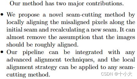
- 解决基于接缝感知的算法得到的接缝有错位的问题。解决方法:SIFTflow+sigmoid平滑。
- 可以将这套体系加入到任何接缝切割方法的框架中。
阅读完代码后,相信你已经对论文有了更深入的理解。那么读懂了之后,你自己写论文的创新点不就来了吗:把本文的图像融合框架加入到你自己方法的框架中。以后的论文涉及到接缝融合,那么基本上就都是这篇了,而不是之前的基于感知的接缝融合算法了。将其他方法应用到你的框架里,是最好的创新方法。Stable Linear Structures and Seam Measurements for Parallax Image Stitching这篇文章不知道大家看没看过,TCSVT的,基本就是没啥创新,把LPC改写了一遍,LPC中没细写的比如Perception-based-seam-cutting,给丰富到论文中了。其实LPC等传统方法的接缝融合都用了Perception-based-seam-cutting。我当时就是看了这篇论文都能中TCSVT我就投的TCSVT,直接被拒了,现在想想水还是太深。但TCSVT初审是真的快,如果你的创新点自己觉得还不错,但又没有那么好,我第一个推荐投TCSVT。
再回顾一下算法:

- 用Perception-based-seam-cutting计算一个初始接缝;
- 用Quality evaluation-based iterative seam estimation for image stitching中提到的SSIM误差评估一下接缝;
- 如果接缝中有错位的像素,则修改;怎么判别呢,就是大于Ostu阈值的就是错位的像素。
- 将错位的像素和块提取出来;
- 用SIFTflow计算两个错位的像素块,得到流向量;
- 用sigmoid函数平滑流向量;
- 根据平滑后的流向量重新对齐之前错位的块;
- 对上面的块重新计算接缝;
- 将修正过的块以及接缝替换原图中的错位的块。
复现一下beta取1,4,8时的不同接缝效果:
beta=1:

beta=4:

beta=8:

初始接缝Perception-based-seam-cutting vs 本文算法修正后:
初始接缝Perception-based-seam-cutting:
本文算法修正后:
可以看到,优化后的接缝明显优于初始的接缝。因为初始的接缝破坏了重叠区域原有的结构(接缝穿过了马路牙子,导致错位),而用本文的算法修正后效果会好很多。
其他的结果留给同学们自己复现吧。
其他想法:经过测试,算法还是有点慢的,考虑能不能提升速度。如果速度能有优势的话,又可以丰富论文内容了。
感谢同学们阅读本文,如果对你有所帮助,点个赞,点个收藏吧,我们下一篇论文源码精读再会!