Qiskit 学习笔记2

进阶电路

Gate类 (qiskit.circuit)

官方文档介绍（包括源码）Gate — Qiskit 0.37.1 documentation

初始化：

from qiskit.circuit import Gate
gt1 = Gate(name="my_gate", num_qubits=2, params=[])

此处name将会在后面绘制出的电路图里显示，num_qubits就是该门需要作为参数的量子比特数

如果要把门添加到某一电路中去，使用append方法：

from qiskit import QuantumRegister, QuantumCircuit
qr1 = QuantumRegister(2)
circ1 = QuantumCircuit(qr1)

circ1.append(gt1, [qr1[0], qr1[1]])
print(circ1.draw())

#       ┌──────────┐
# q0_0: ┤0         ├
#       │  my_gate │
# q0_1: ┤1         ├
#       └──────────┘

子电路 (Subcircuit)

让我们新建一个电路：

qr2 = QuantumRegister(2)
circ2 = QuantumCircuit(qr2)

circ2.h(qr2[1])
circ2.cx(qr2[1],qr2[0])
circ2.name = 'subcircuit_1'

同样地，如果我们想要把一个子电路嵌入另一个电路里，也要使用append方法：

circ1.append(circ2.to_instruction(), [qr1[0], qr1[1]])
print(circ1.draw())
print(circ1.decompose().draw())
#       ┌──────────┐┌───────────────┐
# q0_0: ┤0         ├┤0              ├
#       │  my_gate ││  subcircuit_1 │
# q0_1: ┤1         ├┤1              ├
#       └──────────┘└───────────────┘
#       ┌──────────┐     ┌───┐
# q0_0: ┤0         ├─────┤ X ├
#       │  my_gate │┌───┐└─┬─┘
# q0_1: ┤1         ├┤ H ├──■──
#       └──────────┘└───┘

在绘制电路图时，Qiskit会自动包装电路，如果想要完全展开，需要decompose方法（注意，是函数式编程，不会改变对象本身，展开的电路会被直接返回）

参数化

Parameter类（qiskit.circuit）

初始化及传入参数（传入参数依旧不会改变原电路）：

from qiskit.circuit import Parameter
phi = Parameter('φ')

# phi就像正常角度一样传入即可
circ1.rx(phi, qr1[0])
circ1.cry(phi,qr1[0], qr1[1])

# 绑定参数用 bind_parameters()
print(circ1.bind_parameters({phi: pi/3}).draw())
print(circ1.draw())

#    效果：
#       ┌──────────┐┌───────────────┐┌─────────┐
# q0_0: ┤0         ├┤0              ├┤ RX(π/3) ├─────■─────
#       │  my_gate ││  subcircuit_1 │└─────────┘┌────┴────┐
# q0_1: ┤1         ├┤1              ├───────────┤ RY(π/3) ├
#       └──────────┘└───────────────┘           └─────────┘
#       ┌──────────┐┌───────────────┐┌───────┐
# q0_0: ┤0         ├┤0              ├┤ RX(φ) ├────■────
#       │  my_gate ││  subcircuit_1 │└───────┘┌───┴───┐
# q0_1: ┤1         ├┤1              ├─────────┤ RY(φ) ├
#       └──────────┘└───────────────┘         └───────┘

关于参数化电路有两点需要注意：

• 参数化电路会减少编译损耗(详情: Reducing-compilation-cost)
• 参数化可以像普通电路那样被组合

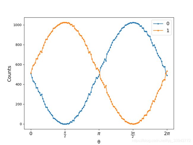
下面看一个综合性的例子：

import matplotlib.pyplot as plt
import numpy as np
from qiskit.circuit import QuantumCircuit, Parameter
from qiskit import BasicAer, execute

backend = BasicAer.get_backend('qasm_simulator')
circuit1 = QuantumCircuit(1, 1)
theta = Parameter('θ')
theta_range = np.linspace(0, 2 * np.pi, 128)

circuit1.h(0)   # 相当于添加了一个初相位 pi/4
circuit1.ry(theta, 0)
circuit1.measure(0, 0)

job = backend.run([circuit1.bind_parameters(theta_val) for theta_val in theta_range])
print(circuit1.draw())
counts = job.result().get_counts()

# 绘图部分
fig = plt.figure(figsize=(8, 6))
ax = fig.add_subplot(111)

ax.plot(theta_range, list(map(lambda c: c.get('0', 0), counts)), '.-', label='0')
ax.plot(theta_range, list(map(lambda c: c.get('1', 0), counts)), '.-', label='1')

ax.set_xticks([i * np.pi / 2 for i in range(5)])
ax.set_xticklabels(['0', r'$\frac{\pi}{2}$', r'$\pi$', r'$\frac{3\pi}{2}$', r'$2\pi$'], fontsize=14)
ax.set_xlabel('θ', fontsize=14)
ax.set_ylabel('Counts', fontsize=14)
ax.legend(fontsize=14)

fig.savefig(r'D:\1.png')

可以这样想象，因为之前在第一篇中提到过，我们选择用来表示态，当对于1个量子态，等价于维空间时，我们可以用一个模长始终为1矢量表示一个量子态。在比较Rx、Ry、Rz三个门后，不难发现Ry正好对应着二维空间中的旋转群，由是便有了上面的例子，我们给定初态为一个夹角为的量子态，之后旋转它（可以从theta_range看出）一步步从0到.结果如下图：

官网有一个略微复杂的实例：Binding parameters to values

操作子

Operator类（qiskit.quantum_info.operaters）

创建和基本属性

每一个Operator实例都包含两个基本属性（继承自BasicOperator） ：

• data：numpy array, 储存操作子的矩阵表示
• dim：操作子的维数信息，不一定和data中的矩阵相同

创建操作子时，只需要提供一个矩阵即可（实际上就是二维列表），无论是不是numpy array都可

操作子维数分为input_dims和output_dims，分别对应的是操作子要施加的量子态数和生成的量子态数，对此官网有如下表述：

For  by   operators, the input and output dimension will be automatically assumed to be M-qubit and N-qubit

谨记，每一个量子比特对应着一个“2”，它们之间用张量积连结 

from qiskit.quantum_info.operators import Operator
import numpy as np

op = Operator(np.random.rand(2 ** 1, 2 ** 2))
print(op.data)   # 会输出随机生成的矩阵 
print(op.dim)    # 输出(4, 2)
print(op.input_dims())    # 输出(2, 2)
print(op.output_dims())    # 输出(2,)

那么对于无法表示成2的幂的维数，qiskit通常不会再处理，例如对于维数为（6, 6）的操作子，其输入维和输出维都是(6,)，但也可以根据张量积将其分解：

op2 = Operator(np.random.rand(4, 6), input_dims=[2, 3], output_dims=[4])
# 2 × 3 = 6
print(op2.output_dims) # 是(4,)而不是(2, 2)

通过实例可见，当指定输出输入维时，不仅原矩阵非2的幂的维数可以被人工分解，还可以避免2的幂的维数被自动分解

相关类型转换

Operator也可以通过Pauli、Gate、Instruction甚至是QuantumCircuit来创建：

from qiskit.circuit.library import HGate

op = Operator(HGate())
print(op)
# Operator([[ 0.70710678+0.j,  0.70710678+0.j],
#           [ 0.70710678+0.j, -0.70710678+0.j]],
#          input_dims=(2,), output_dims=(2,))

需要在电路中使用操作子时，和其他操作一样，调用电路的append()方法并附量子态即可

操作子的组合

张量积对应的两个函数（这里先假设Op1和Op2都是单量子门）：

• op1.tensor(op2) 等价于，其结果还可以表示成一个矩阵，但是在实际作用时，则是Op2对应qubit_0, Op1对应qubit_1
• op1.expand(op2) 等价于

普通的矩阵乘法，调用compose()方法，但和张量积相同，它也在顺序上存在两种形式（矩阵乘法对两矩阵有一定的维数要求）：

• op1.compose(op2)等价于op2·op1
• op1.compose(op2, front=True)等价于op1.op2

子系统乘法

刚才说过普通矩阵乘法会对两矩阵的维数作一定要求，而子系统乘法会将大的矩阵作张量分解，将其拆成若干小矩阵，而我们的目的则是选出那些我们想要作用的小矩阵，结果会自然作张量积变回大矩阵：

op = Operator(np.eye(2 ** 3))
XZ = Operator(Pauli(label='XZ'))
op.compose(XZ, qargs=[0, 2])

（在front参数为False的情况，即默认情况下，调用方应是那个较大的矩阵）

这里可以将op拆成，这三个实际上都是2维单位矩阵，下标用来表示编号，此时我们就可以拿和去和XZ门做普通矩阵乘法（实际上是XZ · I，因为默认front=False）

另外，维数相同的操作子还可以作线性组合

---

欢迎加入Qiskit交流群: 1064371332