【machine learning for everyone 人人都可以学的机器学习】系列文章 1【数据预处理、KNN、朴素贝叶斯、线性回归、SVM、Neural Net】
machine learning for everyone 人人都可以学的机器学习
文章目录
- machine learning for everyone 人人都可以学的机器学习
- 前言
- 数据
- 数据集处理
- 模型相关
-
- kNN
- Naive Bayes
- Log Regression
- svc
- Neural Net
前言
数据集:https://archive.ics.uci.edu/dataset/159/magic+gamma+telescope
数据
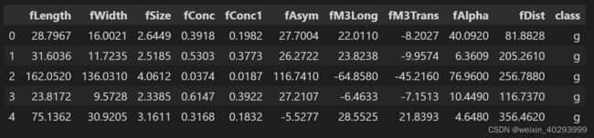
cols = ["fLength", "fWidth", "fSize", "fConc", "fConc1", "fAsym", "fM3Long", "fM3Trans", "fAlpha", "fDist", "class"]
df = pd.read_csv("./dataset/magic04.data",names=cols)
df.head()
df.info()
<class 'pandas.core.frame.DataFrame'>
RangeIndex: 19020 entries, 0 to 19019
Data columns (total 11 columns):
 #   Column    Non-Null Count  Dtype
---  ------    --------------  -----
 0   fLength   19020 non-null  float64
 1   fWidth    19020 non-null  float64
 2   fSize     19020 non-null  float64
 3   fConc     19020 non-null  float64
 4   fConc1    19020 non-null  float64
 5   fAsym     19020 non-null  float64
 6   fM3Long   19020 non-null  float64
 7   fM3Trans  19020 non-null  float64
 8   fAlpha    19020 non-null  float64
 9   fDist     19020 non-null  float64
 10  class     19020 non-null  object
dtypes: float64(10), object(1)
memory usage: 1.6+ MB
class 是两个 g和h
df["class"].unique()
array(['g', 'h'], dtype=object)
将class 数值化
df["class"] = (df["class"]=="g").astype(int)
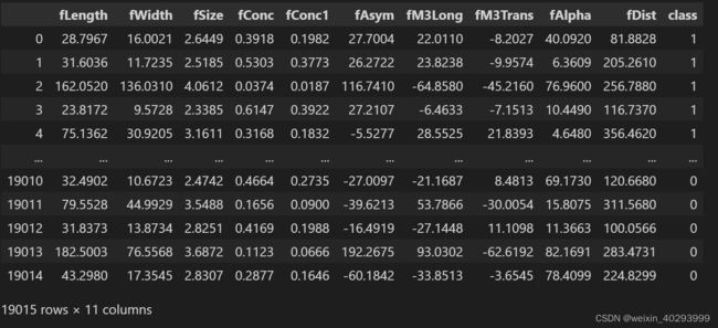
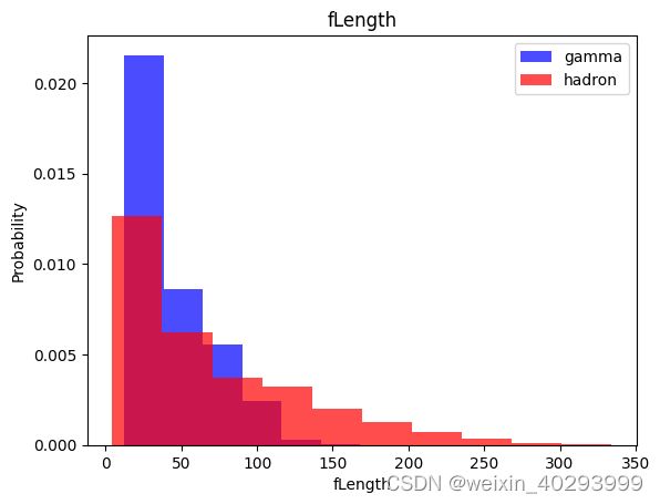
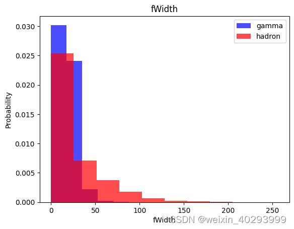
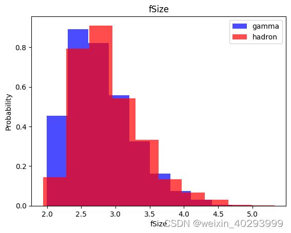
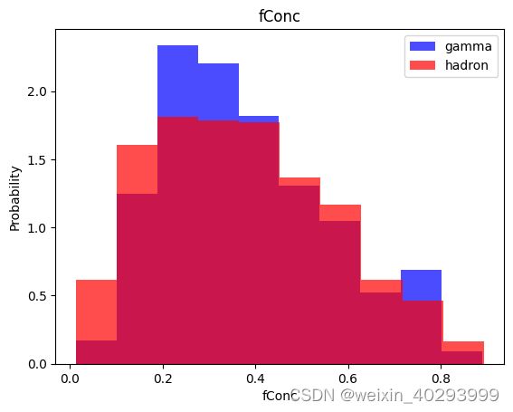
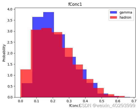
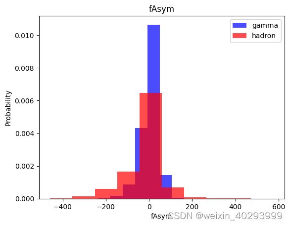
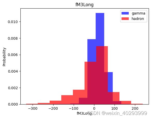
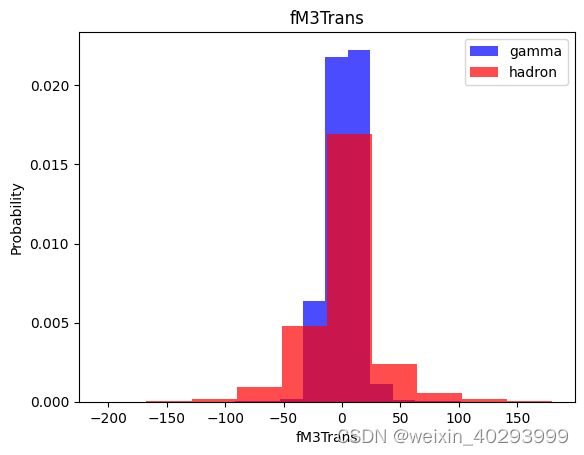
观察数据集
for label in cols[:-1]:
    plt.hist(df[df["class"]==1][label],color ='blue', label='gamma',alpha=0.7,density=True)
    plt.hist(df[df["class"]==0][label],color ='red', label='hadron',alpha=0.7,density=True)
    plt.title(label)
    plt.ylabel("Probability")
    plt.xlabel(label)
    plt.legend()
    plt.show()
数据集处理
Train, validation, test datasets
train, valid, test = np.split(df.sample(frac=1),[int(0.6*len(df)), int(0.8*len(df))])
len(train[train['class']==1]),len(train[train['class']==0])
(7404, 4008)
可以看到数据集不平衡
def scale_dataset(dataframe, oversample=False):
    X = dataframe[dataframe.columns[:-1]].values
    y = dataframe[dataframe.columns[-1]].values
    scaler = StandardScaler()
    X = scaler.fit_transform(X)

    if oversample:
        ros = RandomOverSampler()
        X, y = ros.fit_resample(X,y)

    data = np.hstack((X,np.reshape(y,(-1,1))))
    return data, X,y
train, X_train, y_train = scale_dataset(train, oversample=True)
valid, X_valid, y_valid = scale_dataset(valid, oversample=False)
test, X_test, y_test = scale_dataset(test, oversample=False)
train[:,-1:].sum(),len(train[:,-1:])
(7404.0, 14808)
模型相关
kNN
from sklearn.neighbors import KNeighborsClassifier
from sklearn.metrics import classification_report
knn_model = KNeighborsClassifier(n_neighbors=5)
knn_model.fit(X_train, y_train)
y_pred = knn_model.predict(X_test)
print(classification_report(y_test,y_pred))
              precision    recall  f1-score   support

           0       0.74      0.76      0.75      1365
           1       0.86      0.85      0.86      2439

    accuracy                           0.82      3804
   macro avg       0.80      0.80      0.80      3804
weighted avg       0.82      0.82      0.82      3804
Naive Bayes
from sklearn.naive_bayes import GaussianNB
nb_model = GaussianNB()
nb_model = nb_model.fit(X_train, y_train)
y_pred = nb_model.predict(X_test)
print(classification_report(y_test,y_pred))
             precision    recall  f1-score   support

           0       0.70      0.41      0.51      1365
           1       0.73      0.90      0.81      2439

    accuracy                           0.72      3804
   macro avg       0.71      0.65      0.66      3804
weighted avg       0.72      0.72      0.70      3804
Log Regression
from sklearn.linear_model import LogisticRegression
lg_model = LogisticRegression()
lg_model = lg_model.fit(X_train, y_train)
y_pred = lg_model.predict(X_test)
print(classification_report(y_test, y_pred))
              precision    recall  f1-score   support

           0       0.70      0.73      0.71      1365
           1       0.85      0.82      0.83      2439

    accuracy                           0.79      3804
   macro avg       0.77      0.78      0.77      3804
weighted avg       0.79      0.79      0.79      3804
svc
from sklearn.svm import SVC
svm_model = SVC()
svm_model = svm_model.fit(X_train, y_train)
y_pred = svm_model.predict(X_test)
print(classification_report(y_test, y_pred))
              precision    recall  f1-score   support

           0       0.80      0.80      0.80      1365
           1       0.89      0.89      0.89      2439

    accuracy                           0.86      3804
   macro avg       0.84      0.85      0.85      3804
weighted avg       0.86      0.86      0.86      3804
Neural Net
import tensorflow as tf
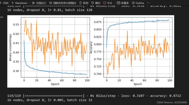
def plot_history(history):
fig, (ax1, ax2) = plt.subplots(1, 2, figsize=(10, 4))
ax1.plot(history.history['loss'], label='loss')
ax1.plot(history.history['val_loss'], label='val_loss')
ax1.set_xlabel('Epoch')
ax1.set_ylabel('Binary crossentropy')
ax1.grid(True)
ax2.plot(history.history['accuracy'], label='accuracy')
ax2.plot(history.history['val_accuracy'], label='val_accuracy')
ax2.set_xlabel('Epoch')
ax2.set_ylabel('Accuracy')
ax2.grid(True)
plt.show()
def train_model(X_train, y_train, num_nodes, dropout_prob, lr, batch_size, epochs):
  nn_model = tf.keras.Sequential([
      tf.keras.layers.Dense(num_nodes, activation='relu', input_shape=(10,)),
      tf.keras.layers.Dropout(dropout_prob),
      tf.keras.layers.Dense(num_nodes, activation='relu'),
      tf.keras.layers.Dropout(dropout_prob),
      tf.keras.layers.Dense(1, activation='sigmoid')
  ])

  nn_model.compile(optimizer=tf.keras.optimizers.Adam(lr), loss='binary_crossentropy',
                  metrics=['accuracy'])
  history = nn_model.fit(
    X_train, y_train, epochs=epochs, batch_size=batch_size, validation_split=0.2, verbose=0
  )

  return nn_model, history
least_val_loss = float('inf')
least_loss_model = None
epochs=100
for num_nodes in [16, 32, 64]:
  for dropout_prob in[0, 0.2]:
    for lr in [0.01, 0.005, 0.001]:
      for batch_size in [32, 64, 128]:
        print(f"{num_nodes} nodes, dropout {dropout_prob}, lr {lr}, batch size {batch_size}")
        model, history = train_model(X_train, y_train, num_nodes, dropout_prob, lr, batch_size, epochs)
        plot_history(history)
        val_loss = model.evaluate(X_valid, y_valid)[0]
        if val_loss < least_val_loss:
          least_val_loss = val_loss
          least_loss_model = model