MATLAB学习QPSK之QPSK_MOD_DEMOD_SALIMup分析

学习的背景说明

因为在学习5G物理层，一直很忙，没有时间。最近稍有一点空闲，所以，学习一下算法。
QPSK的算法，虽然说我没有完全学透，大致还是懂的。只能一直没时间用MATLAB来研究一下。

然后看到这个实例，感觉很好。因为没有中间的AWGN和采样的过程，只讲调制与解调，适合理解。
示例代码见下：

QPSK_MOD_DEMOD_SALIM
MATLAB Code for QPSK Modulation and Demodulation - File Exchange - MATLAB Central
MATLAB Code for QPSK Modulation and Demodulation

Version 1.0.0.0 (2.99 KB) by Md. Salim Raza

MATLAB Code for QPSK Modulation and Demodulation has been Developed According to Conventional Theory

%XXXXXXXXXXXXXXXXXXXXXXXXXXXXXXXXXXXXXXXXXXXXXXXXXXXXXXXXXXXXXXXXXXXXXXXXXX

%XXXX QPSK Modulation and Demodulation without consideration of noise XXXXX

%XXXXXXXXXXXXXXXXXXXXXXXXXXXXXXXXXXXXXXXXXXXXXXXXXXXXXXXXXXXXXXXXXXXXXXXXXX

clc;
clear all;
close all;
data=[0 1 0 1 1 1 0 0 1 1]; % information
%Number_of_bit=1024;
%data=randint(Number_of_bit,1);
figure(1)
stem(data, 'linewidth',3), grid on;
title(' Information before Transmiting ');
axis([ 0 11 0 1.5]);
data_NZR=2*data-1; % Data Represented at NZR form for QPSK modulation
s_p_data=reshape(data_NZR,2,length(data)/2); % S/P convertion of data
br=10.^6; %Let us transmission bit rate 1000000
f=br; % minimum carrier frequency
T=1/br; % bit duration
t=T/99:T/99:T; % Time vector for one bit information
% XXXXXXXXXXXXXXXXXXXXXXX QPSK modulatio XXXXXXXXXXXXXXXXXXXXXXXXXXXXXXXXX
y=[];
y_in=[];
y_qd=[];
for(i=1:length(data)/2)
y1=s_p_data(1,i)*cos(2*pi*f*t); % inphase component
y2=s_p_data(2,i)*sin(2*pi*f*t) ;% Quadrature component
y_in=[y_in y1]; % inphase signal vector
y_qd=[y_qd y2]; %quadrature signal vector
y=[y y1+y2]; % modulated signal vector
end
Tx_sig=y; % transmitting signal after modulation
tt=T/99:T/99:(T*length(data))/2;
figure(2)
subplot(3,1,1);
plot(tt,y_in,'linewidth',3), grid on;
title(' wave form for inphase component in QPSK modulation ');
xlabel('time(sec)');
ylabel(' amplitude(volt0');
subplot(3,1,2);
plot(tt,y_qd,'linewidth',3), grid on;
title(' wave form for Quadrature component in QPSK modulation ');
xlabel('time(sec)');
ylabel(' amplitude(volt0');
subplot(3,1,3);
plot(tt,Tx_sig,'r','linewidth',3), grid on;
title('QPSK modulated signal (sum of inphase and Quadrature phase signal)');
xlabel('time(sec)');
ylabel(' amplitude(volt0');
% XXXXXXXXXXXXXXXXXXXXXXXXXXXX QPSK demodulation XXXXXXXXXXXXXXXXXXXXXXXXXX
Rx_data=[];
Rx_sig=Tx_sig; % Received signal
for(i=1:1:length(data)/2)
%%XXXXXX inphase coherent dector XXXXXXX
Z_in=Rx_sig((i-1)*length(t)+1:i*length(t)).*cos(2*pi*f*t);
% above line indicat multiplication of received & inphase carred signal
Z_in_intg=(trapz(t,Z_in))*(2/T);% integration using trapizodial rull
if(Z_in_intg>0) % Decession Maker
Rx_in_data=1;
else
Rx_in_data=0;
end
%%XXXXXX Quadrature coherent dector XXXXXX
Z_qd=Rx_sig((i-1)*length(t)+1:i*length(t)).*sin(2*pi*f*t);
%above line indicat multiplication ofreceived & Quadphase carred signal
Z_qd_intg=(trapz(t,Z_qd))*(2/T);%integration using trapizodial rull
if (Z_qd_intg>0)% Decession Maker
Rx_qd_data=1;
else
Rx_qd_data=0;
end
Rx_data=[Rx_data Rx_in_data Rx_qd_data]; % Received Data vector
end
figure(3)
stem(Rx_data,'linewidth',3)
title('Information after Receiveing ');
axis([ 0 11 0 1.5]), grid on;
% XXXXXXXXXXXXXXXXXXXXXXXXX end of program XXXXXXXXXXXXXXXXXXXXXXXXXX

运行的结果如图
单步跟踪代码后，基本都能理解。
特别是调制的部分，都比较熟悉：
S(t)=I⋅cos(2πft)+Q⋅sin(2πft)
这里稍加注意，中国的教科书，大多I与Q是正负相反的，也就是在空间的旋转方向相反；但国外，包括wiki百科，都是相加的，也就是同向。
matlab，显然是同向的，所以是相加。
但是到解调时，就有些看不懂了。

这一句：
Z_in_intg=(mytrapz(t,Z_in))(2/T);% integration using trapizodial rull
为什么积分是>0或者<0，而不是等于0?
这里我研究了好半天。
最后发现是这样的：
调制时，这一句：
y1= s_p_data(1,i)cos(2pift); % inphase component
将一个信号，例如这里是1，乘以cos(2pift)。
可以简单理解为将直流信号，装到一个cos的载波上。
解调时，先：
Z_in=Rx_sig((i-1)length(t)+1:ilength(t)).cos(2pift);
待解的符号，再次乘以cos(2pif*t);
这样就得到了cos的平方。
从而积分值>0 或者 <0，而不是等于零。

同样,Q路信号,调制和解调,分别被乘以一次sin ,所以是sin的平方。所以，积分不再是零。

如下图，将第一个IQ数据改为： data=[-5 1]; % information
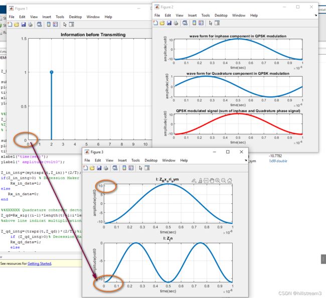第一次将图形输出出来之后，没有看懂的原因，如上图，没有看Y轴坐标，还以为是从-1到正1，其坐标已经变了。都在X轴之上，或之下。积分自然不再是零。

附：改之后，用于学习的调试代码

%XXXXXXXXXXXXXXXXXXXXXXXXXXXXXXXXXXXXXXXXXXXXXXXXXXXXXXXXXXXXXXXXXXXXXXXXXX
%XXXX QPSK Modulation and Demodulation without consideration of noise XXXXX
%XXXXXXXXXXXXXXXXXXXXXXXXXXXXXXXXXXXXXXXXXXXXXXXXXXXXXXXXXXXXXXXXXXXXXXXXXX


clc;
clear all;
close all;
% data=[0 0 1 0 1 1 0 1]; % information
% data=[0 1 1 0 1 1 0 0]; % information
data=[-1 1]; % information
%Number_of_bit=1024;
%data=randint(Number_of_bit,1);

figure(1)
stem(data, 'linewidth',3), grid on;
title('  Information before Transmiting ');
axis([ 0 11 0 1.5]);

data_NZR=2*data-1; % Data Represented at NZR form for QPSK modulation
s_p_data=reshape(data_NZR,2,length(data)/2);  % S/P convertion of data


br=10.^6; %Let us transmission bit rate  1000000
f=br; % minimum carrier frequency
T=1/br; % bit duration
t=T/99:T/99:T; % Time vector for one bit information



% XXXXXXXXXXXXXXXXXXXXXXX QPSK modulatio  XXXXXXXXXXXXXXXXXXXXXXXXXXXXXXXXX
y=[];
y_in=[];
y_qd=[];
for(i=1:length(data)/2)    
    y1= s_p_data(1,i)*cos(2*pi*f*t); % inphase component
    y2=s_p_data(2,i)*sin(2*pi*f*t) ;% Quadrature component
    y_in=[y_in y1]; % inphase signal vector
    y_qd=[y_qd y2]; %quadrature signal vector
    y=[y y1+y2]; % modulated signal vector
end
Tx_sig=y1; % transmitting signal after modulation
tt=T/99:T/99:(T*length(data))/2;

figure(2)

subplot(3,1,1);
plot(tt,y_in,'linewidth',3), grid on;
title(' wave form for inphase component in QPSK modulation ');
xlabel('time(sec)');
ylabel(' amplitude(volt0');

subplot(3,1,2);
plot(tt,y_qd,'linewidth',3), grid on;
title(' wave form for Quadrature component in QPSK modulation ');
xlabel('time(sec)');
ylabel(' amplitude(volt0');


subplot(3,1,3);
plot(tt,Tx_sig,'r','linewidth',3), grid on;
title('QPSK modulated signal (sum of inphase and Quadrature phase signal)');
xlabel('time(sec)');
ylabel(' amplitude(volt0');




% XXXXXXXXXXXXXXXXXXXXXXXXXXXX QPSK demodulation XXXXXXXXXXXXXXXXXXXXXXXXXX
figure(3)
Rx_data=[];
Rx_sig=Tx_sig; % Received signal
for(i=1:1:length(data)/2)

    
    Z_Rx_ori_sym=Rx_sig((i-1)*length(t)+1:i*length(t));
    
    subplot(2,1,1);
    plot(t,Z_Rx_ori_sym,'linewidth',3), grid on;
    title('I: Z_Rx_ori_sym ');
    xlabel('time(sec)');
    ylabel(' amplitude(volt0');
    
    %%XXXXXX inphase coherent dector XXXXXXX
    Z_in=Rx_sig((i-1)*length(t)+1:i*length(t)).*cos(2*pi*f*t); 
    %Z_in=Rx_sig((i-1)*length(t)+1:i*length(t)); 
    % above line indicat multiplication of received & inphase carred signal
    
    subplot(2,1,2);
    plot(t,Z_in,'linewidth',3), grid on;
    title('I: Z_in');
    xlabel('time(sec)');
    ylabel(' amplitude(volt0');

    Z_in_intg=(mytrapz(t,Z_in))*(2/T);% integration using trapizodial rull
    if(Z_in_intg>0) % Decession Maker
        Rx_in_data=1;
    else
       Rx_in_data=0; 
    end
    
    %%XXXXXX Quadrature coherent dector XXXXXX
    Z_qd=Rx_sig((i-1)*length(t)+1:i*length(t)).*sin(2*pi*f*t);
    %above line indicat multiplication ofreceived & Quadphase carred signal
    
    Z_qd_intg=(trapz(t,Z_qd))*(2/T);%integration using trapizodial rull
        if (Z_qd_intg>0)% Decession Maker
        Rx_qd_data=1;
        else
       Rx_qd_data=0; 
        end
        
        
        Rx_data=[Rx_data  Rx_in_data  Rx_qd_data]; % Received Data vector
end


figure(4)
stem(Rx_data,'linewidth',3) 
title('Information after Receiveing ');
axis([ 0 11 0 1.5]), grid on;


% XXXXXXXXXXXXXXXXXXXXXXXXX    end of program    XXXXXXXXXXXXXXXXXXXXXXXXXX