深度学习与python theano
文章目录
- 前言
-
- 1.人工神经网络
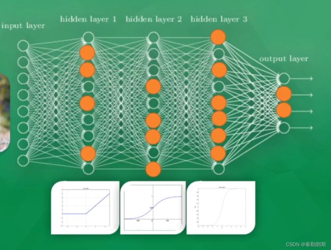
- 2.计算机神经网络
- 3.反向传播
- 4.梯度下降-cost 函数
-
- 1.一维
- 2.二维
- 3.局部最优
- 4.迁移学习
- 5. theano-GPU-CPU
- theano介绍
- 1.安装
- 2.基本用法
-
- 1.回归
- 2.分类
- 3.function用法
- 4.shared 变量
- 5.activation function
- 6.Layer层
- 7.regression 回归例子
- 8.classification分类学习
- 9.过拟合
- 10.正则化
- 11.save model
- 12 总结
前言
本章主要介绍深度学习与python theano。
主要整理来自B站:
1.深度学习框架简介 Theano
2.Theano python 神经网络
1.人工神经网络
2.计算机神经网络
3.反向传播
4.梯度下降-cost 函数
1.一维
2.二维
3.局部最优
大部分时间我们只能求得一个局部最优解
4.迁移学习
5. theano-GPU-CPU
tenforflow鼻祖
theano介绍
1.安装
win10安装theano
设置
ldflags = -lblas
window10安装,这里要说明一点的是python3.8安装theano会出现一些非常奇怪的问题,所以这里选用python3.7.
conda create -n theano_env python=3.7
conda activate theano_env
conda install numpy scipy mkl-service libpython m2w64-toolchain


#如果想要安装的快点,可以使用国内的镜像
pip install -i https://pypi.tuna.tsinghua.edu.cn/simple theano
安装后出现了下列问题:
WARNING (theano.tensor.blas): Failed to import scipy.linalg.blas, and Theano flag blas.ldflags is empty. Falling back on slower implementations for dot(matrix, vector), dot(vector, matrix) and dot(vector, vector) (DLL load failed: 找不到指定的模块。)
不过想了一下,自己也只是学习一下而已,慢就慢吧,不用C的
2.基本用法
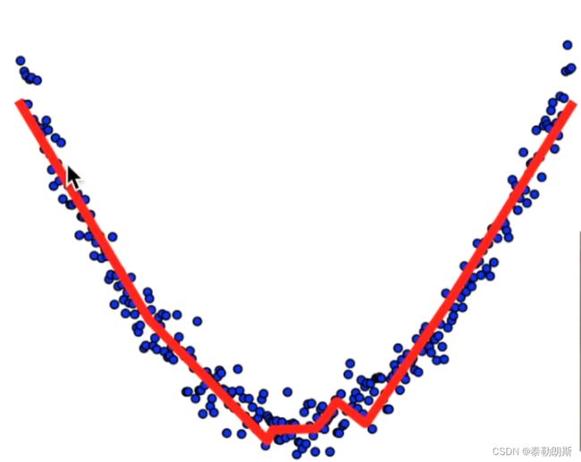
1.回归
拟合曲线
# View more python tutorials on my Youtube and Youku channel!!!

# Youtube video tutorial: https://www.youtube.com/channel/UCdyjiB5H8Pu7aDTNVXTTpcg
# Youku video tutorial: http://i.youku.com/pythontutorial

# 10 - visualize result
"""
Please note, this code is only for python 3+. If you are using python 2+, please modify the code accordingly.
"""
from __future__ import print_function
import theano
import theano.tensor as T
import numpy as np
import matplotlib.pyplot as plt


class Layer(object):
    def __init__(self, inputs, in_size, out_size, activation_function=None):
        self.W = theano.shared(np.random.normal(0, 1, (in_size, out_size)))
        self.b = theano.shared(np.zeros((out_size, )) + 0.1)
        self.Wx_plus_b = T.dot(inputs, self.W) + self.b
        self.activation_function = activation_function
        if activation_function is None:
            self.outputs = self.Wx_plus_b
        else:
            self.outputs = self.activation_function(self.Wx_plus_b)


# Make up some fake data
x_data = np.linspace(-1, 1, 300)[:, np.newaxis]
noise = np.random.normal(0, 0.05, x_data.shape)
y_data = np.square(x_data) - 0.5 + noise        # y = x^2 - 0.5

# show the fake data
plt.scatter(x_data, y_data)
plt.show()

# determine the inputs dtype
x = T.dmatrix("x")
y = T.dmatrix("y")

# add layers
l1 = Layer(x, 1, 10, T.nnet.relu)
l2 = Layer(l1.outputs, 10, 1, None)

# compute the cost
cost = T.mean(T.square(l2.outputs - y))

# compute the gradients
gW1, gb1, gW2, gb2 = T.grad(cost, [l1.W, l1.b, l2.W, l2.b])

# apply gradient descent
learning_rate = 0.05
train = theano.function(
    inputs=[x, y],
    outputs=[cost],
    updates=[(l1.W, l1.W - learning_rate * gW1),
             (l1.b, l1.b - learning_rate * gb1),
             (l2.W, l2.W - learning_rate * gW2),
             (l2.b, l2.b - learning_rate * gb2)])

# prediction
predict = theano.function(inputs=[x], outputs=l2.outputs)

# plot the real data
fig = plt.figure()
ax = fig.add_subplot(1,1,1)
ax.scatter(x_data, y_data)
plt.ion()
plt.show()

for i in range(1000):
    # training
    err = train(x_data, y_data)
    if i % 50 == 0:
        # to visualize the result and improvement
        try:
            ax.lines.remove(lines[0])
        except Exception:
            pass
        prediction_value = predict(x_data)
        # plot the prediction
        lines = ax.plot(x_data, prediction_value, 'r-', lw=5)
        plt.pause(.5)