基于keras采用LSTM实现多标签文本分类(一)
多标签和多分类的区别
1.多标签即一条语句可能有多个类别划分。例如,这个酸菜鱼又酸又辣。属于酸和辣两个标签。
在采用神经网络学习时,最后一层的激活函数应采用sigmoid激活函数,相当于对这条语句做了多个二分类。
2.多分类即每条语句只有一个标签,在采用神经网络学习时,最后一层的激活函数应采用softmax激活函数,最后选取类别中的最大值作为预测结果。
关于sigmoid和softmax 的区别此处再说明。
本次数据集的格式为:
组织关系-裁员 消失的“外企光环”,5月份在华裁员900余人,香饽饽变“臭”了
组织关系-裁员 前两天,被称为“仅次于苹果的软件服务商”的Oracle(甲骨文)公司突然宣布在中国裁员。。
组织关系-裁员 不仅仅是中国IT企业在裁员,为何500强的甲骨文也发生了全球裁员
关于LSTM的学习可以参考这篇。
关于词向量化的方式,本文采用keras 内置Tokenizer API 实现。
运行环境tensorflow2,keras 2.+
from tensorflow.keras.preprocessing.text import Tokenizer
from tensorflow.keras.preprocessing.sequence import pad_sequences
import re
import jieba
from sklearn.preprocessing import MultiLabelBinarizer
from tensorflow.keras.models import Model, load_model
from tensorflow.keras.layers import *
import numpy as np
import json
def clear_character(sentence):
pattern1 = '[a-zA-Z0-9]'
pattern2 = re.compile(u'[^\s1234567890' + '\u4e00-\u9fa5]+')
pattern3 = '[’!"#$%&\'()*+,-./:;<=>?@[\\]^_`{|}~]+【】'
line1 = re.sub(pattern1, '', sentence)
line2 = re.sub(pattern2, '', line1)
line3 = re.sub(pattern3, '', line2)
new_Sentence = ''.join(line3.split())
return new_Sentence
def content_split(segment):
seg = " ".join(jieba.cut(segment))
return seg
def rm_stop_word(wordlist, stop):
filtered_words = [word for word in wordlist if word not in stop]
return filtered_words
def get_all_labels():
labels = []
for _ in train_content + test_content:
label = _.split(" ")[0].split("|")
for __ in label:
if __ not in labels:
labels.append(__)
return labels
def write_to_json(label_list):
with open("data/event_type.json", "w", encoding="utf-8") as h:
h.write(json.dumps(label_list, ensure_ascii=False, indent=4))
with open("./data/multi-classification-train.txt", "r", encoding="utf-8") as f:
train_content = [_.strip() for _ in f.readlines()]
with open("./data/multi-classification-test.txt", "r", encoding="utf-8") as f:
test_content = [_.strip() for _ in f.readlines()]
with open('./data/stopWord.json', 'r', encoding='utf-8') as f:
stop_word = [_.strip() for _ in f.readlines()]
genders = get_all_labels()
# write_to_json(genders)
# 获取训练文本集和训练标签集
train_data = []
train_label = []
for line in train_content:
genres = line.split(" ", maxsplit=1)[0].split("|")
co = line.split(" ", maxsplit=1)[1]
train_data.append(co)
train_label.append(genres)
# 标签向量化
mutil_lab = MultiLabelBinarizer()
train_label = mutil_lab.fit_transform(train_label)
# 移除无用字符
train_content_remove = []
for content in train_data:
train_content_remove.append(clear_character(content))
# 利用jieba分词
train_content_split = []
for string in train_content_remove:
train_content_split.append(content_split(string))
# 去除停用词
train_content_stop = rm_stop_word(train_content_split, stop_word)
# 训练集的文本处理也是一样的
test_data = []
test_label = []
for line in test_content:
genres = line.split(" ", maxsplit=1)[0].split("|")
co = line.split(" ", maxsplit=1)[1]
test_data.append(co)
test_label.append(genres)
test_content_remove = []
for content in test_data:
test_content_remove.append(clear_character(content))
mutil_lab = MultiLabelBinarizer()
test_label = mutil_lab.fit_transform(test_label)
test_content_split = []
for string in test_content_remove:
test_content_split.append(content_split(string))
test_content_stop = rm_stop_word(test_content_split, stop_word)
print(test_content_stop[0:5])
# 利用Tokenizer 向量化文本
tokenizer = Tokenizer(num_words=40000, filters='!"#$%&()*+,-./:;<=>?@[\]^_`{|}~', lower=True)
tokenizer.fit_on_texts(train_content_stop)
x_data = tokenizer.texts_to_sequences(train_content_stop)
x_data = pad_sequences(x_data, 100)
y_data = np.array(train_label)
print("训练集的大小为: ", x_data.shape, "训练集标签的大小为: ", y_data.shape)
x_test_data = tokenizer.texts_to_sequences(test_content_stop)
x_test_data = pad_sequences(x_test_data, 100)
y_test_data = np.array(test_label)
print("测试集的大小为: ", x_test_data.shape, "测试集标签的大小为: ", y_test_data.shape)
# 训练集的大小为: (11958, 100) 训练集标签的大小为: (11958, 65)
# 测试集的大小为: (1498, 100) 测试集标签的大小为: (1498, 65)
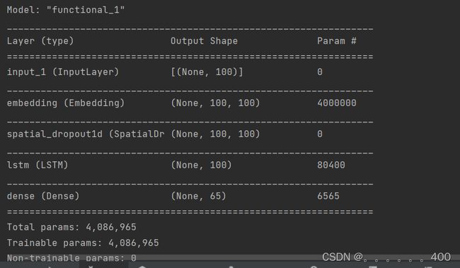
# 构建模型
inputs = Input(shape=(100,))
embed = Embedding(40000, 100, input_length=x_data.shape[1])(inputs)
dropout = SpatialDropout1D(0.2)(embed)
lstm = LSTM(100, dropout=0.2, recurrent_dropout=0, activation='tanh', recurrent_activation='sigmoid')(dropout) # 注意LSTM层的参数是为了能够用上cuDNN的加速
output = Dense(y_data.shape[1], activation='sigmoid')(lstm)
model = Model(inputs, output)
model.compile(loss='binary_crossentropy', optimizer='adam', metrics=['accuracy'])
model.summary()
history = model.fit(x_data, y_data, batch_size=16, epochs=20, validation_data=(x_test_data, y_test_data))
model.save("lstm.h5")
模型搭建如下:
运行结果部分截图为:
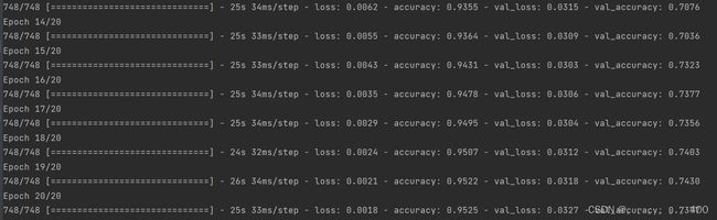
可以看到训练集准确率为95%,验证集为74%。接下来的工作可以采用Word2vec,Bert等模型向量化文本,或者采用双层LSTM看看结果如何。