具有神经网络思维的Logistic回归
**
1 - Packages(导入包,加载数据集)
1.1导入包
其中,用到的Python包有:
◎numpy 是使用Python进行科学计算的基础包。
◎h5py Python提供读取HDF5二进制数据格式文件的接口,本次的训练及测试图片集是以HDF5储存的。
◎matplotlib 是Python中著名的绘图库。
◎PIL (Python Image Library) 为 Python提供图像处理功能。
◎scipy 基于NumPy来做高等数学、信号处理、优化、统计和许多其它科学任务的拓展库。
导入包编程实现:
import numpy as np                   #numpy 是使用Python进行科学计算的基础包。
import matplotlib.pyplot as plt      #是Python中著名的绘图库。
import h5py                          #基于NumPy来做高等数学、信号处理、优化、统计和许多其它科学任务的拓展库。
import scipy                         ##ython提供读取HDF5二进制数据格式文件的接口,本次的训练及测试图片集是以HDF5储存的。
from PIL import Image                #(Python Image Library) 为 Python提供图像处理功能
from scipy import ndimage
from lr_utils import load_dataset    # 用来导入数据集的
#%matplotlib inline   #设置matplotlib在行内显示图片
1.2加载数据包
新建文件lr_utils.py
#温馨提示:如果该作业在本地运行,该数据集的代码保存在lr_utils.py文件,并和当前项目保存在一个文件夹下
加载数据集编程实现:
2 - Overview of the Problem set(目标:预处理数据)
2.1 导入数据
编程实现:
import numpy as np
import h5py
"""
    train_set_x_orig :保存的是训练集里面的图像数据(本训练集有209张64x64的图像)。
    train_set_y_orig :保存的是训练集的图像对应的分类值(【0 | 1】,0表示不是猫,1表示是猫)。
    test_set_x_orig :保存的是测试集里面的图像数据(本训练集有50张64x64的图像)。
    test_set_y_orig : 保存的是测试集的图像对应的分类值(【0 | 1】,0表示不是猫,1表示是猫)。
    classes : 保存的是以bytes类型保存的两个字符串数据,数据为:[b’non-cat’ b’cat’]。
"""
#HDF5文件是一种存储dataset 和 group 两类数据对象的容器,其操作类似 python 标准的文件操作;File 实例对象本身就是一个组,以 / 为名,是遍历文件的入口。
#h5py.File(文件名,可以是字节字符串或 unicode 字符串, 'mode')
def load_dataset():
    train_dataset = h5py.File('datasets/train_catvnoncat.h5', "r")
    train_set_x_orig = np.array(train_dataset["train_set_x"][209])
    train_set_y_orig = np.array(train_dataset["train_set_y"][:])

    test_dataset = h5py.File('datasets/test_catvnoncat.h5', "r")
    test_set_x_orig = np.array(test_dataset["test_set_x"][:])
    test_set_y_orig = np.array(test_dataset["test_set_y"][:])

    classes = np.array(test_dataset["list_classes"][:])

    train_set_y_orig = train_set_y_orig.reshape((1, train_set_y_orig.shape[0]))
    test_set_y_orig = test_set_y_orig.reshape((1, test_set_y_orig.shape[0]))

    return train_set_x_orig, train_set_y_orig, test_set_x_orig, test_set_y_orig, classes
2.2 测试数据 编程实现:
#测试数据
index = 25 #标签数目
plt.imshow(train_set_x_orig[index])
print ("y = " + str(train_set_y_orig[:,index]) + ", it's a '" + classes[np.squeeze(test_set_y_orig[:,index])].decode("utf-8") +  "' picture.")
编程输出:
![]()
2.3计算训练集、测试集的大小以及图像的大小
编程实现:
#计算训练集、测试集的大小以及图像的大小
m_train = train_set_y_orig.shape[1]
m_test = test_set_y_orig.shape[1]
num_px = train_set_x_orig.shape[1]
print ("Number of training examples: m_train = " + str(m_train))
print ("Number of testing examples: m_test = " + str(m_test))
print ("Height/Width of each image: num_px = " + str(num_px))
print ("Each image is of size: (" + str(num_px) + ", " + str(num_px) + ", 3)")
print ("train_set_x shape: " + str(train_set_x_orig.shape))
print ("train_set_y shape: " + str(train_set_y_orig.shape))
print ("test_set_x shape: " + str(test_set_x_orig.shape))
print ("test_set_y shape: " + str(test_set_y_orig.shape))
编程结果:

2.4 转换矩阵
整个训练集转为一个矩阵,其中包括num_pxnum_py3行,m_train列。
其中X_flatten = X.reshape(X.shape[0], -1).T可以:将一个维度为(a,b,c,d)的矩阵转换为一个维度为(b∗c∗d, a)的矩阵。
编程实现:
#转化矩阵
#整个训练集转为一个矩阵,其中包括num_pxnum_py3行,m_train列
train_set_x_flatten = train_set_x_orig.reshape(train_set_x_orig.shape[0],-1).T
test_set_x_flatten = test_set_x_orig.reshape(test_set_x_orig.shape[0], -1).T
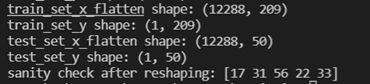
print ("train_set_x_flatten shape: " + str(train_set_x_flatten.shape))
print ("train_set_y shape: " + str(train_set_y_orig.shape))
print ("test_set_x_flatten shape: " + str(test_set_x_flatten.shape))
print ("test_set_y shape: " + str(test_set_y_orig.shape))
print ("sanity check after reshaping: " + str(train_set_x_flatten[0:5,0]))
编程结果:
2.5预处理数据(去中心化)
为了表示图像(RGB)必须指定为每个像素,实际上像素值就是三个数字组成的向量(0-255))
通常机器学习的预处理工作是去中心化和标准化你的数据集,(x - mean)/标准差。但是对图像数据集,数据集的每一行除以255(最大值的像素通道)更简单方便高效)
编程实现:
#去中心化
train_set_x = train_set_x_flatten / 255
test_set_x = test_set_x_flatten / 255
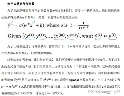
代价函数和成本知识补充:


3 - Building the parts of our algorithm(构建算法的部分)
搭建一个神经网络的主要步骤:
- 定义模型结构(例如输入特征的数量)
- 初始化模型的参数
- 循环操作
计算当前的 loss 值(前向传播)
计算当前的梯度值(反向传播)
更新参数,梯度下降算法
3.1 - sigmod()函数实现
实现sigmod()函数, 你需要计算sigmoid(wTx+b)来进行预测
编程实现:
#sigmoid()函数实现
def sigmoid(z):
    """
    Compute the sigmoid of z

    Arguments:
    x -- A scalar or numpy array of any size.

    Return:
    s -- sigmoid(z)
    """
    s = 1 / (1 + np.exp(-z))
return s
print ("sigmoid(0) = " + str(sigmoid(0)))
print ("sigmoid(9.2) = " + str(sigmoid(9.2)))
编程结果:
![]()
3.2 - 初始化参数(w, b)
在下面实现参数初始化。你不得不初始化w为一个零向量。使用np.zeros().
编程实现:
# 初始化参数(w, b)
def initialize_with_zeros(dim):
"""
This function creates a vector of zeros of shape (dim, 1) for w and initializes b to 0.
Argument:
dim -- size of the w vector we want (or number of parameters in this case)
Returns:
w -- initialized vector of shape (dim, 1)
b -- initialized scalar (corresponds to the bias)
"""
w = np.zeros(shape=(dim, 1)) # 初始化 w 为 (dim行,1列) 的向量
b = 0
assert(w,shape == (dim, 1)) # 判断 w 的shape是否为 (dim, 1), 不是则终止程序
assert(isinstance(b, float) or isinstance(b, int)) # 判断 b 是否是float或者int类型
return w, b
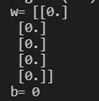
w,b = initialize_with_zeros(5)
print("w=", w)
print("b=", b)
编程结果:
3.3 - 前向传播和后向传播
现在你的参数已经初始化,可以进行 前向传播和后向传播步骤来学习参数。
实现一个函数 ropagate() 来计算 代价函数 和 他的梯度
编程实现:
# 前向传播和后向传播
def propagate(w, b, X, Y):
"""
Implement the cost function and its gradient for the propagation explained above
Arguments:
w -- weights, a numpy array of size (num_px * num_px * 3, 1)
b -- bias, a scalar
X -- data of size (num_px * num_px * 3, number of examples)
Y -- true "label" vector (containing 0 if non-cat, 1 if cat) of size (1, number of examples)
Return:
cost -- negative log-likelihood cost for logistic regression
dw -- gradient of the loss with respect to w, thus same shape as w
db -- gradient of the loss with respect to b, thus same shape as b
Tips:
- Write your code step by step for the propagation
"""
m = X.shape[1] #样例个数
# 前向传播(Forward Propagation)
A = sigmoid(np.dot(w.T, X) + b) # 计算 activation , A 的 维度是 (m, m)
cost = (- 1 / m) * np.sum(Y * np.log(A) + (1 - Y) * (np.log(1 - A))) # 计算 cost; Y == yhat(1, m)
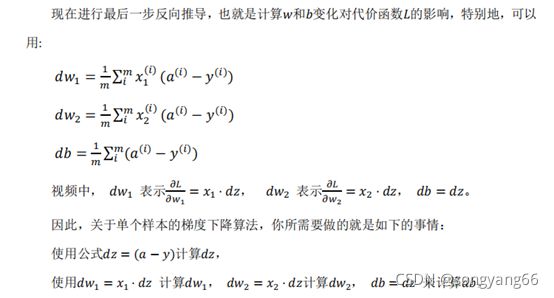
# 反向传播(Backward Propagation)
dw = (1 / m) * np.dot(X, (A - Y).T) # 计算 w 的导数
db = (1 / m) * np.sum(A - Y) # 计算 b 的导数
assert(dw.shape == w.shape) # 减少bug出现
assert(db.dtype == float) # db 是一个值
cost = np.squeeze(cost) # 压缩维度,(从数组的形状中删除单维条目,即把shape中为1的维度去掉),保证cost是值
assert(cost.shape == ())
grads = {"dw": dw,
"db": db}
return grads, cost
w, b, X, Y = np.array([[1], [2]]), 2, np.array([[1,2], [3,4]]), np.array([[1, 0]])
grads, cost = propagate(w, b, X, Y)
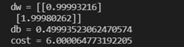
print ("dw = " + str(grads["dw"]))
print ("db = " + str(grads["db"]))
print ("cost = " + str(cost))
编程结果:
3.4 Optimization(最优化)
已初始化了你的参数。
已经能够计算一个代价函数和他的梯度。
现在需要用梯度下降算法更新参数。
写下 optimization function(优化函数),目标是通过最小化代价函数 J,学习参数w和 b。对参数θ,更新规则是θ=θ– αdθ,α是 learning rate)
编程实现:
#Optimization(最优化)
def optimize(w, b, X, Y, num_iterations, learning_rate, print_cost = False):
"""
This function optimizes w and b by running a gradient descent algorithm
Arguments:
w -- weights, a numpy array of size (num_px * num_px * 3, 1)
b -- bias, a scalar
X -- data of shape (num_px * num_px * 3, number of examples)
Y -- true "label" vector (containing 0 if non-cat, 1 if cat), of shape (1, number of examples)
num_iterations -- number of iterations of the optimization loop 优化循环的迭代次数
learning_rate -- learning rate of the gradient descent update rule
print_cost -- True to print the loss every 100 steps
Returns:
params -- 包含权重w和偏差b的字典
grads -- 字典包含权重的梯度和相对于代价函数的偏差
costs -- 在优化过程中计算的所有成本的列表,这将用于绘制学习曲线.
小贴士:
你基本上需要写下两个步骤并迭代它们:
1)计算当前参数的代价和梯度。使用传播()。
2)对w和b使用梯度下降规则更新参数。
"""
costs = []
for i in range(num_iterations):
# Cost and gradient calculation(成本和梯度计算)
grads, cost = propagate(w, b, X, Y)
# Retrieve derivatives from grads(获取导数)
dw = grads["dw"]
db = grads["db"]
# update rule (更新 参数)
w = w - learning_rate * dw # need to broadcast
b = b - learning_rate * db
# Record the costs (每一百次记录一次 cost)
if i % 100 == 0:
costs.append(cost)
# Print the cost every 100 training examples (如果需要打印则每一百次打印一次)
if print_cost and i % 100 == 0:
print ("Cost after iteration %i: %f" % (i, cost))
# 记录 迭代好的参数 (w, b)
params = {"w": w,
"b": b}
# 记录当前导数(dw, db), 以便下次继续迭代
grads = {"dw": dw,
"db": db}
return params, grads, costs
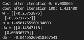
params, grads, costs = optimize(w, b, X, Y, num_iterations= 200, learning_rate = 0.009, print_cost = True)
print ("w = " + str(params["w"]))
print ("b = " + str(params["b"]))
print ("dw = " + str(grads["dw"]))
print ("db = " + str(grads["db"]))
编程结果:
3.5预测函数
前面的函数 将输出学习好的参数 (w, b), 我们可以使用w和b来预测数据集 x 的标签,实现 predict() 函数。计算预测有两个步骤:
- 计算 Y_hat = A = sigmod(w.T X + b)
- 转换 a 为 0 (如果 activation <= 0.5) 或者 1 (如果activation > 0.5),存储预测值在 向量Y_prediction中。如果你想,你可以在for循环中使用 if/else(尽管有方法将其向量化)
编程实现:
#预测函数 predict
#1. 计算 Y_hat = A = sigmod(w.T X + b)
#2. 转换 a 为 0 (如果 activation <= 0.5) 或者 1 (如果activation > 0.5),存储预测值在 向量Y_prediction中
def predict(w, b, X):
    '''
    Predict whether the label is 0 or 1 using learned logistic regression parameters (w, b)
    Arguments:
    w -- weights, a numpy array of size (num_px * num_px * 3, 1)
    b -- bias, a scalar
    X -- data of size (num_px * num_px * 3, number of examples)
    Returns:
    Y_prediction -- a numpy array (vector) containing all predictions (0/1) for the examples in X
    '''
    m = X.shape[1]
    Y_prediction = np.zeros((1, m))
    w = w.reshape(X.shape[0], 1)

    # 计算向量A,预测图片中出现一只猫的概率
    A = sigmoid(np.dot(w.T, X) + b)
    for i in range(A.shape[1]):
        # 将概率a[0,i]转换为实际预测p[0,i]
        Y_prediction[0, i] = 1 if A[0, i] > 0.5 else 0

    assert(Y_prediction.shape == (1, m))

    return Y_prediction
print("predictions = " + str(predict(w, b, X)))
编程结果:
![]()
4 - 合并所有函数在一个model()里
你将看到如何通过将所有构建(在前面部分中实现的功能)按照正确的顺序组合在一起来构建整个模型。
步骤:
Y_prediction :你在测试集上进行预测
Y_prediction_train:你在训练集上的预测
w, costs, grads :optimize()的输出
编程实现:
# 合并所有函数在一个model()里
def model(X_train, Y_train, X_test, Y_test, num_iterations=2000, learning_rate=0.5, print_cost=False):
"""
Builds the logistic regression model by calling the function you've implemented previously
Arguments:
X_train -- 训练集training set represented by a numpy array of shape (num_px * num_px * 3, m_train)
Y_train -- 训练标签training labels represented by a numpy array (vector) of shape (1, m_train)
X_test -- test set represented by a numpy array of shape (num_px * num_px * 3, m_test)
Y_test -- test labels represented by a numpy array (vector) of shape (1, m_test)
num_iterations -- hyperparameter representing the number of iterations to optimize the parameters
learning_rate -- hyperparameter representing the learning rate used in the update rule of optimize()
print_cost -- Set to true to print the cost every 100 iterations
Returns:
d -- dictionary containing information about the model.包含关于模型的信息的字典
"""
# initialize parameters with zeros (初始化参数(w, b))
w, b = initialize_with_zeros(X_train.shape[0]) # num_px*num_px*3
# Gradient descent (前向传播和后向传播 同时 梯度下降更新参数)
parameters, grads, costs = optimize(w, b, X_train, Y_train, num_iterations, learning_rate, print_cost)
# Retrieve parameters w and b from dictionary "parameters"(获取参数w, b)
w = parameters["w"]
b = parameters["b"]
# Predict test/train set examples (使用测试集和训练集进行预测)
Y_prediction_train = predict(w, b, X_train)
Y_prediction_test = predict(w, b, X_test)
# Print train/test Errors (训练/测试误差: (100 - mean(abs(Y_hat - Y))*100 )
print("train accuracy: {} %".format(100 - np.mean(np.abs(Y_prediction_train - Y_train)) * 100))
print("test accuracy: {} %".format(100 - np.mean(np.abs(Y_prediction_test - Y_test)) * 100))
d = {"costs": costs,
"Y_prediction_test": Y_prediction_test,
"Y_prediction_train" : Y_prediction_train,
"w" : w,
"b" : b,
"learning_rate" : learning_rate,
"num_iterations": num_iterations}
return d
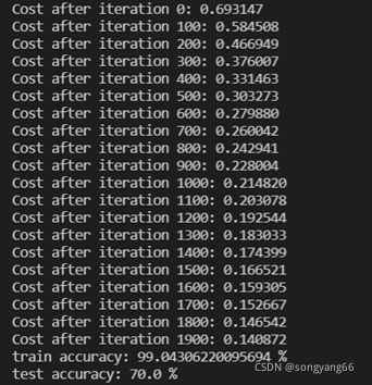
d = model(train_set_x, train_set_y_orig, test_set_x, test_set_y_orig, num_iterations = 2000, learning_rate = 0.005, print_cost = True)
编程结果:
5-成本图绘制和学习率选择
5.1成本图
成本在下降表明参数正则学习中。可以在训练集对模型进行更多的培训。尝试增加以上代码中的迭代次数,并重新运行代码,训练集的准确性会提高,但是测试集的精度会下降。这就是过渡拟合。
编程实现:
#Plot learning curve (with costs) 绘制成本图
iterations = np.array(np.squeeze(d['iterations']))
print("iterations===",iterations)
costs = np.array(np.squeeze(d['costs']))
print("costs===",costs)
plt.plot(iterations,costs)
plt.ylabel('cost')
plt.xlabel('iterations (per hundreds)')
plt.title("Learning rate =" + str(d["learning_rate"]))
plt.show()
编程结果:

5.2学习率
选择一个learning rate α
Reminder:为了让梯度下降能够工作,你必须明智的选择learning rate α。α决定了我们更新参数的速度。如果学习率太高,我们可能会”超过”最优值。同样,如果他太小,我们将需要太多的迭代来收敛到最佳值。这就是为什么使用良好α至关重要。
让我们比较我们的模型的α与几种选择的α。
编程实现:
#改变学习率调试
learning_rates = [0.01, 0.001, 0.0001]
models = {}

for i in learning_rates:
    print ("learning rate is: " + str(i))
    models[str(i)] = model(train_set_x, train_set_y_orig, test_set_x, test_set_y_orig, num_iterations = 1500, learning_rate = i, print_cost = False)
    print ('\n' + "-------------------------------------------------------" + '\n')

for i in learning_rates:
    plt.plot(np.squeeze(models[str(i)]["costs"]), label= str(models[str(i)]["learning_rate"]))

plt.ylabel('cost')
plt.xlabel('iterations')

legend = plt.legend(loc='upper center', shadow=True)
frame = legend.get_frame()
frame.set_facecolor('0.90')
plt.show()
编程结果:
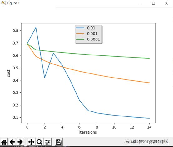
分析:
• 不同α带来不同的cost,因此不同预测结果
• 如果学习率太高(0.01),cost可能上下波。(尽管本例中0.01还行)
• 更低的成本不意味着一个更好的模型。你需要检查一下是否可能过拟合。当训练精度远远高于测试精度时,就会过拟合!
• 在深度学习中,我们推荐
o 选择能够更好最小化代价的 learning rate
o 如果模型过拟合,选择其他技术减少过拟合
lr_utils.py代码:
import numpy as np
import h5py
"""
    train_set_x_orig :保存的是训练集里面的图像数据(本训练集有209张64x64的图像)。
    train_set_y_orig :保存的是训练集的图像对应的分类值(【0 | 1】,0表示不是猫,1表示是猫)。
    test_set_x_orig :保存的是测试集里面的图像数据(本训练集有50张64x64的图像)。
    test_set_y_orig : 保存的是测试集的图像对应的分类值(【0 | 1】,0表示不是猫,1表示是猫)。
    classes : 保存的是以bytes类型保存的两个字符串数据,数据为:[b’non-cat’ b’cat’]。
"""

#温馨提示:如果该作业在本地运行,该数据集的代码保存在lr_utils.py文件,并和当前项目保存在一个文件夹下

#HDF5文件是一种存储dataset 和 group 两类数据对象的容器,其操作类似 python 标准的文件操作;File 实例对象本身就是一个组,以 / 为名,是遍历文件的入口。
#h5py.File(文件名,可以是字节字符串或 unicode 字符串, 'mode')
def load_dataset():
    train_dataset = h5py.File('datasets/train_catvnoncat.h5', "r")
    train_set_x_orig = np.array(train_dataset["train_set_x"][:]) # your train set features
    train_set_y_orig = np.array(train_dataset["train_set_y"][:]) # your train set labels

    test_dataset = h5py.File('datasets/test_catvnoncat.h5', "r")
    test_set_x_orig = np.array(test_dataset["test_set_x"][:]) # your test set features
    test_set_y_orig = np.array(test_dataset["test_set_y"][:]) # your test set labels

    classes = np.array(test_dataset["list_classes"][:]) # the list of classes

    train_set_y_orig = train_set_y_orig.reshape((1, train_set_y_orig.shape[0]))
    test_set_y_orig = test_set_y_orig.reshape((1, test_set_y_orig.shape[0]))

    return train_set_x_orig, train_set_y_orig, test_set_x_orig, test_set_y_orig, classes
主程序代码:
import numpy as np                   #numpy 是使用Python进行科学计算的基础包。
import matplotlib.pyplot as plt      #是Python中著名的绘图库。
import h5py
from numpy.core.fromnumeric import shape                          #基于NumPy来做高等数学、信号处理、优化、统计和许多其它科学任务的拓展库。
import scipy                         ##ython提供读取HDF5二进制数据格式文件的接口,本次的训练及测试图片集是以HDF5储存的。
from PIL import Image                #(Python Image Library) 为 Python提供图像处理功能
from scipy import ndimage
from lr_utils import load_dataset    # 用来导入数据集的
#%matplotlib inline   #设置matplotlib在行内显示图片

#温馨提示:如果该作业在本地运行,该数据集的代码保存在lr_utils.py文件,并和当前项目保存在一个文件夹下
"""
    train_set_x_orig :保存的是训练集里面的图像数据(本训练集有209张64x64的图像)。
    train_set_y_orig :保存的是训练集的图像对应的分类值(【0 | 1】,0表示不是猫,1表示是猫)。
    test_set_x_orig :保存的是测试集里面的图像数据(本训练集有50张64x64的图像)。
    test_set_y_orig : 保存的是测试集的图像对应的分类值(【0 | 1】,0表示不是猫,1表示是猫)。
    classes : 保存的是以bytes类型保存的两个字符串数据,数据为:[b’non-cat’ b’cat’]。
"""
#导入数据
train_set_x_orig, train_set_y_orig, test_set_x_orig, test_set_y_orig, classes = load_dataset()
"""
#测试数据
index = 25 #标签数目
plt.imshow(train_set_x_orig[index])
print ("y = " + str(train_set_y_orig[:,index]) + ", it's a '" + classes[np.squeeze(test_set_y_orig[:,index])].decode("utf-8") +  "' picture.")
"""
#计算训练集、测试集的大小以及图像的大小
m_train = train_set_y_orig.shape[1]
m_test = test_set_y_orig.shape[1]
num_px = train_set_x_orig.shape[1]
print ("Number of training examples: m_train = " + str(m_train))
print ("Number of testing examples: m_test = " + str(m_test))
print ("Height/Width of each image: num_px = " + str(num_px))
print ("Each image is of size: (" + str(num_px) + ", " + str(num_px) + ", 3)")
print ("train_set_x shape: " + str(train_set_x_orig.shape))
print ("train_set_y shape: " + str(train_set_y_orig.shape))
print ("test_set_x shape: " + str(test_set_x_orig.shape))
print ("test_set_y shape: " + str(test_set_y_orig.shape))

#转化矩阵
#整个训练集转为一个矩阵,其中包括num_px*num_py*3行,m_train列
train_set_x_flatten = train_set_x_orig.reshape(train_set_x_orig.shape[0],-1).T
test_set_x_flatten = test_set_x_orig.reshape(test_set_x_orig.shape[0], -1).T

print ("train_set_x_flatten shape: " + str(train_set_x_flatten.shape))
print ("train_set_y shape: " + str(train_set_y_orig.shape))
print ("test_set_x_flatten shape: " + str(test_set_x_flatten.shape))
print ("test_set_y shape: " + str(test_set_y_orig.shape))
print ("sanity check after reshaping: " + str(train_set_x_flatten[0:5,0]))

#去中心化
train_set_x = train_set_x_flatten / 255
test_set_x = test_set_x_flatten / 255

#sigmoid()函数实现
def sigmoid(z):
    """
    Compute the sigmoid of z

    Arguments:
    x -- A scalar or numpy array of any size.

    Return:
    s -- sigmoid(z)
    """
    s = 1 / (1 + np.exp(-z))
    return s
"""
print ("sigmoid(0) = " + str(sigmoid(0)))
print ("sigmoid(9.2) = " + str(sigmoid(9.2)))
"""
# 初始化参数(w,  b)
def initialize_with_zeros(dim):
    """
    This function creates a vector of zeros of shape (dim, 1) for w and initializes b to 0.

    Argument:
    dim -- size of the w vector we want (or number of parameters in this case)参数的数量

    Returns:
    w -- initialized vector of shape (dim, 1)
    b -- initialized scalar (corresponds to the bias)
    """
    w = np.zeros(shape=(dim, 1))    # 初始化 w 为 (dim行,1列) 的向量
    b = 0
    assert(w,shape == (dim, 1))   # 判断 w 的shape是否为 (dim, 1), 不是则终止程序
    assert(isinstance(b, float) or isinstance(b, int))   # 判断 b 是否是float或者int类型

    return w, b
"""
w,b = initialize_with_zeros(5)
print("w=", w)
print("b=", b)
"""
# 前向传播和后向传播
def propagate(w, b, X, Y):
    """
    Implement the cost function and its gradient for the propagation explained above

    Arguments:
    w -- weights, a numpy array of size (num_px * num_px * 3, 1)
    b -- bias, a scalar
    X -- data of size (num_px * num_px * 3, number of examples)
    Y -- true "label" vector (containing 0 if non-cat, 1 if cat) of size (1, number of examples)

    Return:
    cost -- negative log-likelihood cost for logistic regression
    dw -- gradient of the loss with respect to w, thus same shape as w
    db -- gradient of the loss with respect to b, thus same shape as b

    Tips:
    - Write your code step by step for the propagation
    """
    m = X.shape[1]      #样例个数

    # 前向传播(Forward Propagation)
    A = sigmoid(np.dot(w.T, X) + b) # 计算 activation , A 的 维度是 (m, m)
    cost = (- 1 / m) * np.sum(Y * np.log(A) + (1 - Y) * (np.log(1 - A)))  # 计算 cost; Y == yhat(1, m)
    # 反向传播(Backward Propagation)
    dw = (1 / m) * np.dot(X, (A - Y).T) # 计算 w 的导数
    db = (1 / m) * np.sum(A - Y)          # 计算 b 的导数

    assert(dw.shape == w.shape)          # 减少bug出现
    assert(db.dtype == float)            # db 是一个值
    cost = np.squeeze(cost)              # 压缩维度,(从数组的形状中删除单维条目,即把shape中为1的维度去掉),保证cost是值
    assert(cost.shape == ())

    grads = {"dw": dw,
             "db": db}

    return grads, cost
"""
w, b, X, Y = np.array([[1], [2]]), 2, np.array([[1,2], [3,4]]), np.array([[1, 0]])
grads, cost = propagate(w, b, X, Y)
print ("dw = " + str(grads["dw"]))
print ("db = " + str(grads["db"]))
print ("cost = " + str(cost))
"""
#Optimization(最优化)
def optimize(w, b, X, Y, num_iterations, learning_rate, print_cost = False):
    """
    This function optimizes w and b by running a gradient descent algorithm

    Arguments:
    w -- weights, a numpy array of size (num_px * num_px * 3, 1)
    b -- bias, a scalar
    X -- data of shape (num_px * num_px * 3, number of examples)
    Y -- true "label" vector (containing 0 if non-cat, 1 if cat), of shape (1, number of examples)
    num_iterations -- number of iterations of the optimization loop  优化循环的迭代次数
    learning_rate -- learning rate of the gradient descent update rule
    print_cost -- True to print the loss every 100 steps

    Returns:
    params -- 包含权重w和偏差b的字典
    grads -- 字典包含权重的梯度和相对于代价函数的偏差
    costs -- 在优化过程中计算的所有成本的列表,这将用于绘制学习曲线.

    小贴士:
    你基本上需要写下两个步骤并迭代它们:
        1)计算当前参数的代价和梯度。使用传播()。
        2)对w和b使用梯度下降规则更新参数。
    """
    iterations = []
    costs = []
    for i in range(num_iterations):

        # Cost and gradient calculation(成本和梯度计算)
        grads, cost = propagate(w, b, X, Y)
        # Retrieve derivatives from grads(获取导数)
        dw = grads["dw"]
        db = grads["db"]

        # update rule (更新 参数)
        w = w - learning_rate * dw  # need to broadcast
        b = b - learning_rate * db

        # Record the costs (每一百次记录一次 cost)
        if i % 100 == 0:
            iterations.append(i)
            costs.append(cost)
        # Print the cost every 100 training examples (如果需要打印则每一百次打印一次)
        if print_cost and i % 100 == 0:
            print ("Cost after iteration %i: %f" % (i, cost))

    # 记录 迭代好的参数 (w, b)
    params = {"w": w,
              "b": b}

    # 记录当前导数(dw, db), 以便下次继续迭代
    grads = {"dw": dw,
             "db": db}

    return params, grads, costs, iterations
"""
params, grads, costs = optimize(w, b, X, Y, num_iterations= 200, learning_rate = 0.009, print_cost = True)
print ("w = " + str(params["w"]))
print ("b = " + str(params["b"]))
print ("dw = " + str(grads["dw"]))
print ("db = " + str(grads["db"]))
"""
#预测函数 predict
#1.	计算 Y_hat = A = sigmod(w.T X + b)
#2.	转换 a 为 0 (如果 activation <= 0.5) 或者 1 (如果activation > 0.5),存储预测值在 向量Y_prediction中
def predict(w, b, X):
    '''
    Predict whether the label is 0 or 1 using learned logistic regression parameters (w, b)
    Arguments:
    w -- weights, a numpy array of size (num_px * num_px * 3, 1)
    b -- bias, a scalar
    X -- data of size (num_px * num_px * 3, number of examples)
    Returns:
    Y_prediction -- a numpy array (vector) containing all predictions (0/1) for the examples in X
    '''
    m = X.shape[1]
    Y_prediction = np.zeros((1, m))
    w = w.reshape(X.shape[0], 1)

    # 计算向量A,预测图片中出现一只猫的概率
    A = sigmoid(np.dot(w.T, X) + b)
    for i in range(A.shape[1]):
        # 将概率a[0,i]转换为实际预测p[0,i]
        Y_prediction[0, i] = 1 if A[0, i] > 0.5 else 0

    assert(Y_prediction.shape == (1, m))

    return Y_prediction
#print("predictions = " + str(predict(w, b, X)))

# 合并所有函数在一个model()里
def model(X_train, Y_train, X_test, Y_test, num_iterations=2000, learning_rate=0.5, print_cost=False):
    """
    Builds the logistic regression model by calling the function you've implemented previously

    Arguments:
    X_train -- 训练集training set represented by a numpy array of shape (num_px * num_px * 3, m_train)
    Y_train -- 训练标签training labels represented by a numpy array (vector) of shape (1, m_train)
    X_test -- test set represented by a numpy array of shape (num_px * num_px * 3, m_test)
    Y_test -- test labels represented by a numpy array (vector) of shape (1, m_test)
    num_iterations -- hyperparameter representing the number of iterations to optimize the parameters
    learning_rate -- hyperparameter representing the learning rate used in the update rule of optimize()
    print_cost -- Set to true to print the cost every 100 iterations

    Returns:
    d -- dictionary containing information about the model.包含关于模型的信息的字典
    """
    # initialize parameters with zeros (初始化参数(w, b))
    w, b = initialize_with_zeros(X_train.shape[0])         # num_px*num_px*3

    # Gradient descent (前向传播和后向传播 同时 梯度下降更新参数)
    parameters, grads, costs, iterations = optimize(w, b, X_train, Y_train, num_iterations, learning_rate, print_cost)
    print("iterations",iterations)
    # Retrieve parameters w and b from dictionary "parameters"(获取参数w, b)
    w = parameters["w"]
    b = parameters["b"]

    # Predict test/train set examples (使用测试集和训练集进行预测)
    Y_prediction_train = predict(w, b, X_train)
    Y_prediction_test = predict(w, b, X_test)

    # Print train/test Errors (训练/测试误差: (100 - mean(abs(Y_hat - Y))*100 )
    print("train accuracy: {} %".format(100 - np.mean(np.abs(Y_prediction_train - Y_train)) * 100))
    print("test accuracy: {} %".format(100 - np.mean(np.abs(Y_prediction_test - Y_test)) * 100))

    d = {"costs": costs,
         "iterations": iterations,
         "Y_prediction_test": Y_prediction_test,
         "Y_prediction_train" : Y_prediction_train,
         "w" : w,
         "b" : b,
         "learning_rate" : learning_rate,
         "num_iterations": num_iterations}

    return d

d = model(train_set_x, train_set_y_orig, test_set_x, test_set_y_orig, num_iterations = 2000, learning_rate = 0.005, print_cost = True)

#图片分类错误的例子
index = 5
#plt.imshow(test_set_x[:,index].reshape((num_px, num_px, 3)))
#test_set_y[0, index]:测试集里标签;  classes[int(d["Y_Prediction_test"][0, index])]:预测值
print ("y = " + str(test_set_y_orig[0, index]) + ", you predicted that it is a \"" + classes[int(d["Y_prediction_test"][0, index])].decode("utf-8") +  "\" picture.")
#Plot learning curve (with costs) 绘制成本图
iterations = np.array(np.squeeze(d['iterations']))
print("iterations===",iterations)
costs = np.array(np.squeeze(d['costs']))
print("costs===",costs)
plt.plot(iterations,costs)
plt.ylabel('cost')
plt.xlabel('iterations (per hundreds)')
plt.title("Learning rate =" + str(d["learning_rate"]))
plt.show()

#改变学习率调试
learning_rates = [0.01, 0.001, 0.0001]
models = {}
for i in learning_rates:
    print ("learning rate is: " + str(i))
    models[str(i)] = model(train_set_x, train_set_y_orig, test_set_x, test_set_y_orig, num_iterations = 1500, learning_rate = i, print_cost = False)
    print ('\n' + "-------------------------------------------------------" + '\n')
for i in learning_rates:
    plt.plot(np.squeeze(models[str(i)]["costs"]), label= str(models[str(i)]["learning_rate"]))

plt.ylabel('cost')
plt.xlabel('iterations')

legend = plt.legend(loc='upper center', shadow=True)
frame = legend.get_frame()
frame.set_facecolor('0.90')
plt.show()
资源链接:https://www.cnblogs.com/douzujun/p/10267165.html
资源链接:https://blog.csdn.net/u013733326/article/details/79827273
文件下载:https://download.csdn.net/download/songyang66/45702882