GEMMA 全基因组关联分析+CMplot多性状曼哈顿+QQ图脚本

GEMMA 全基因组关联分析+CMplot多性状曼哈顿+QQ图脚本

###GEMMA 全基因组关联分析+CMplot多性状曼哈顿+QQ图脚本
#作者：刘济铭

##########################
GWAS理论和基本结果理解已经有很多大神进行了解读，因此不再赘述，想要学习请移步知乎或各大基因课平台学习。本人发现目前缺乏具体实用脚本，因此本帖只提供本人脚本供大家交流学习，本人脚本不是最好肯定也会存在问题，请大家见谅。

###全基因组关联分析前需对SNP文件利用repeatmodeler和repeatmasker去除重复片段，后续分析均采用去重复片段SNP文件分析。
#vcftools 过滤VCF文件
vcftools --vcf testnorepeats.recode.vcf --min-alleles 2 --max-alleles 2 --maf 0.05 --max-missing 0.3  --minQ 20 --recode --out test
#此步骤根据各自需求决定，去除多余vcf文件中多余个体数据，id.txt自行构建，个体名按列排布即可
vcftools --vcf test.recode.vcf --recode --recode-INFO-all --stdout  --remove id.txt   > out.vcf
#转plink bed，ped文件
vcftools   --vcf out.vcf --plink --out testnorepeat
plink --file testnorepeat   --make-bed --out testnorepeat --noweb

## 下载GEMMA
wget -c https://github.com/genetics-statistics/GEMMA/releases/download/0.98.1/gemma-0.98.1-linux-static.gz
## 解压
gzip -d gemma-0.98.1-linux-static.gz
## 设置权限
chmod a+x gemma-0.98.1-linux-static

##！！！！！计算亲缘关系矩阵前必须将plink所得fam文件第六列及以后添加各个体相对应表型数据，后续关联分析用-n定位哪个表型，-n 1 为第六列表型分析，-n 2 为第七列表型分析，以此类推

##运行gemma
####计算亲缘关系矩阵，-bfile：输入Plink二进制格式文件的前缀。-gk：指定生成的kinship矩阵类型。
#-gk 1 为centered matrix，-gk 2 为standardized matrix。
#-o：输出文件前缀。
./gemma-0.98.1-linux-static -bfile testnorepeat -gk 2 -o kinship
#运行gemma关联分析，可利用-a输入参考基因组基因注释gff3文件
./gemma-0.98.1-linux-static -bfile testnorepeat -k ./output/kinship.sXX.txt -n 39 -a final.gene.gff3  -lmm 4 -o out

#完成关联分析

#利用CMplot R包实现曼哈顿图和qq图制作

##首先在linux系统中提取gwas分析结果文件中1,2,3,13列数据
cut -f 1,2,3,13 out.assoc.txt  > out1.assoc.txt

#对换第1列和第二列位置
awk '{print $2,$1,$3,$4}' out1.assoc.txt > out2.assoc.txt

###利用vim工具更改表头为SNP Chromosome Position Trait1 Trait2 Trait3。。。。。。。

###此时out2.assoc.txt为R CMplot作图输入文件

#### 计算GWAS显著关联SNP位点阈值，此处采用Bonferroni correction = 显著性水平（0.01/0.05）/ Me Me为去冗余独立SNP数量，可使用plink --file testnorepeat --r 指令得到，也可自行设定阈值范围
###！！！以下阈值为本人数据计算结果，大家请自行根据数据计算更改后使用
cat out.assoc.txt  | awk -F ' '  '$13<5.78e-09{print $0}' > out.top1.out
cat out.assoc.txt  | awk -F ' '  '$13<2.89e-08{print $0}' > out.top5.out

###提取SNP位置信息
awk  '{print $1"\t"$3}' out.top1.out  >  out1.snp.position
awk  '{print $1"\t"$3}' out.top5.out  >  out5.snp.position
###提取SNP上下游各50kb范围，范围可根据各自数据LD或自行参考文献确定
awk 'BEGIN{FS=OFS="\t"}{if(NR>1){ print $1,$2-50000,$2+50000 }}' out1.snp.position | sort -k 1,1 -k 2,2n  > out1.snp.bed
awk 'BEGIN{FS=OFS="\t"}{if(NR>1){ print $1,$2-50000,$2+50000 }}' out5.snp.position | sort -k 1,1 -k 2,2n  > out5.snp.bed
#####利用bedtools merge工具实现位置重叠SNP融合
bedtools merge -i out1.snp.bed > out1.snpmerged.bed
bedtools merge -i out5.snp.bed > out5.snpmerged.bed

###注意，所得out1.snpmerged.bed可能存在染色体名称与参考基因组注释文件差异，务必统一为参考基因组注释文件染色体名称形式，不然无法获得交叉对比结果

#awk  '{print $1"\t"$4"\t"$5"\t"$9}' gene.gff3  >  gene_after.gff3

###利用bedtools intersect工具实现显著SNP位点上下游50kb内基因交叉对比提取
bedtools intersect -a /scratch/n2007039f/output/gene.gff3  -b out1.snpmerged.bed -wa > gene_top1.out

bedtools intersect -a /scratch/n2007039f/output/gene.gff3  -b out5.snpmerged.bed -wa > gene_top5.out

####检查数据，查看第13列从小到大情况
###less out.assoc.txt|sort -k 13g|less


####R中CMplot包实现GWASQQ图，曼哈顿图等的单个和多个表型联合作图multi_plot
cut -f 13 out.assoc.txt  > LAD
paste FHD FLD.txt FVD.txt > 1
######better to set all Tab to Space
sed 's/\t/ /g' 1 > 2
#使用R作图，建议服务器中使用，计算容量较大
## 加载R包
library("CMplot")
## 导入数据
data <- read.table("out2.assoc.txt",sep=" ",header=T)
#SNP-density plot

CMplot(data,type="p",plot.type="d",bin.size=1e6,chr.den.col=c("darkgreen", "yellow", "red"),file="jpg",memo="",dpi=300,
    main="illumilla_60K",file.output=TRUE,verbose=TRUE,width=9,height=6)
	
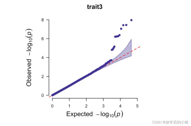
## 绘制单个表型Q-Q plot
CMplot(data,plot.type="q",conf.int=TRUE,box=FALSE,file="jpg",memo="",dpi=300,file.output=TRUE,verbose=TRUE,width=5,height=5)

## 绘制单个表型Rectangular-Manhattan plot，注意threshold设置，不同数据集不同阈值设置
CMplot(data,plot.type="m",LOG10=TRUE,threshold=5.78e-09,file="tif",memo="",dpi=500,file.output=TRUE,verbose=TRUE,width=18,height=8,signal.col=NULL)

CMplot(data,plot.type="m",LOG10=TRUE,threshold=2.89e-08,file="tif",memo="",dpi=500,file.output=TRUE,verbose=TRUE,width=18,height=8,signal.col=NULL)


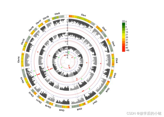
#Genome-wide association study(GWAS)多表型作图，注意threshold设置，不同数据集不同阈值设置
CMplot(data,type="p",plot.type="c",chr.labels=paste("Chr",c(1:14),sep=""),r=0.4,cir.legend=TRUE,
        outward=FALSE,cir.legend.col="black",cir.chr.h=1.3,chr.den.col="black",file="jpg",
        memo="",dpi=300,file.output=TRUE,verbose=TRUE,width=10,height=10)
		
CMplot(data,type="p",plot.type="c",r=0.4,col=c("grey30","grey60"),chr.labels=paste("Chr",c(1:14),sep=""),
      threshold=c(5.78e-09,2.89e-08),cir.chr.h=1.5,amplify=TRUE,threshold.lty=c(1,2),threshold.col=c("red",
      "blue"),signal.line=1,signal.col=c("red","green"),chr.den.col=c("darkgreen","yellow","red"),
      bin.size=1e6,outward=FALSE,file="jpg",memo="",dpi=300,file.output=TRUE,verbose=TRUE,width=10,height=10)
####manhatton plot
CMplot(data, plot.type="m", LOG10=TRUE, ylim=NULL, threshold=c(5.78e-09,2.89e-08),threshold.lty=c(1,2),
        threshold.lwd=c(1,1), threshold.col=c("black","grey"), amplify=TRUE,bin.size=1e6,
        chr.den.col=c("darkgreen", "yellow", "red"),signal.col=c("red","green"),signal.cex=c(1.5,1.5),
        signal.pch=c(19,19),file="jpg",memo="",dpi=300,file.output=TRUE,verbose=TRUE,
        width=14,height=6)
#####Multi_tracks Q-Q plot
CMplot(data,plot.type="q",box=FALSE,file="jpg",memo="",dpi=300,
    conf.int=TRUE,conf.int.col=NULL,threshold.col="red",threshold.lty=2,
    file.output=TRUE,verbose=TRUE,width=5,height=5)

部分成图结果展示：

CMplot包参考学习来源：https://github.com/YinLiLin/CMplot，感谢Lilin Yin大神的CMplot包。
CMplot包Author: Lilin Yin
Contact: [email protected]
QQ group: 166305848
Institution: Huazhong agricultural university