yolov5部分loss部分代码解析
文章目录
- 前言
前言
主要是关于loss计算的代码,之前阅读了几篇博主的文章,并观察了代码的每一步结果,现在谈一下自己对这部分代码的理解。
1. build_targets
#这里na为锚框种类数 nt为目标数 这里的na为3,nt也为3
na, nt = self.na, targets.shape[0]  # number of anchors, targets
#类别 边界盒 索引 锚框
tcls, tbox, indices, anch = [], [], [], []
#利用gain来计算目标在某一个特征图上的位置信息,初始化为1
gain = torch.ones(7, device=targets.device)  # normalized to gridspace gain
# ai.shape = (na, nt),锚框的索引,三个目标,三种锚框,所以共9个元素
ai = torch.arange(na, device=targets.device).float().view(na, 1).repeat(1, nt)  # same as .repeat_interleave(nt)
Out[3]:
tensor([[0., 0., 0.],
        [1., 1., 1.],
        [2., 2., 2.]], device='cuda:0')
# targets.shape = (na, nt, 7)(3,3,7)给每个目标加上锚框索引
#targets[i,c,x,y,w,h,锚框索引]
targets = torch.cat((targets.repeat(na, 1, 1), ai[:, :, None]), 2)
Out[4]:
tensor([[[0.00000, 0.00000, 0.58192, 0.16796, 0.26108, 0.08724, 0.00000],
         [1.00000, 0.00000, 0.54517, 0.33744, 0.06395, 0.02632, 0.00000],
         [1.00000, 0.00000, 0.96964, 0.42483, 0.06071, 0.05264, 0.00000]],
        [[0.00000, 0.00000, 0.58192, 0.16796, 0.26108, 0.08724, 1.00000],
         [1.00000, 0.00000, 0.54517, 0.33744, 0.06395, 0.02632, 1.00000],
         [1.00000, 0.00000, 0.96964, 0.42483, 0.06071, 0.05264, 1.00000]],
        [[0.00000, 0.00000, 0.58192, 0.16796, 0.26108, 0.08724, 2.00000],
         [1.00000, 0.00000, 0.54517, 0.33744, 0.06395, 0.02632, 2.00000],
         [1.00000, 0.00000, 0.96964, 0.42483, 0.06071, 0.05264, 2.00000]]], device='cuda:0')
g = 0.5  # bias
#off偏移量(不知道这么称合适吗)
off = torch.tensor([[0, 0],
                            [1, 0], [0, 1], [-1, 0], [0, -1],  # j,k,l,m
                            # [1, 1], [1, -1], [-1, 1], [-1, -1],  # jk,jm,lk,lm
                            ], device=targets.device).float() * g  # offsets
#off的形状如下,为什么是这个形状下文解释
Out[5]:
tensor([[ 0.00000,  0.00000],
        [ 0.50000,  0.00000],
        [ 0.00000,  0.50000],
        [-0.50000,  0.00000],
        [ 0.00000, -0.50000]], device='cuda:0')
for i in range(self.nl):

"""
p[i].shape = (b, 3, h, w,nc+5)
gain = [1, 1, w, h, w, h, 1]

nl->number of layer,检测特征图
"""#获取当前的锚框尺寸
    anchors = self.anchors[i]
Out[7]:
tensor([[1.25000, 1.62500],
        [2.00000, 3.75000],
        [4.12500, 2.87500]], device='cuda:0')
    gain[2:6] = torch.tensor(p[i].shape)[[3, 2, 3, 2]]  # xyxy gain
Out[8]: tensor([ 1.,  1., 64., 64., 64., 64.,  1.], device='cuda:0')
    # 将xywh映射到当前特征图,即乘以对应的特征图尺寸
    # Match targets to anchors
    t = targets * gain #
Out[9]:
tensor([[[ 0.00000,  0.00000, 37.24281, 10.74930, 16.70916,  5.58366,  0.00000],
         [ 1.00000,  0.00000, 34.89063, 21.59622,  4.09269,  1.68436,  0.00000],
         [ 1.00000,  0.00000, 62.05726, 27.18916,  3.88548,  3.36872,  0.00000]],
        [[ 0.00000,  0.00000, 37.24281, 10.74930, 16.70916,  5.58366,  1.00000],
         [ 1.00000,  0.00000, 34.89063, 21.59622,  4.09269,  1.68436,  1.00000],
         [ 1.00000,  0.00000, 62.05726, 27.18916,  3.88548,  3.36872,  1.00000]],
        [[ 0.00000,  0.00000, 37.24281, 10.74930, 16.70916,  5.58366,  2.00000],
         [ 1.00000,  0.00000, 34.89063, 21.59622,  4.09269,  1.68436,  2.00000],
         [ 1.00000,  0.00000, 62.05726, 27.18916,  3.88548,  3.36872,  2.00000]]], device='cuda:0')#t(3,3,7)
    if nt:
        #r为目标wh和锚框wh的比值,比值在0.25到4即采用该种锚框预测目标
        r = t[:, :, 4:6] / anchors[:, None]
Out[10]:
tensor([[[13.36733,  3.43610],
         [ 3.27415,  1.03653],
         [ 3.10838,  2.07306]],
        [[ 8.35458,  1.48897],
         [ 2.04635,  0.44916],
         [ 1.94274,  0.89833]],
        [[ 4.05071,  1.94214],
         [ 0.99217,  0.58587],
         [ 0.94193,  1.17173]]], device='cuda:0')
        #将比值和预先设置的比例anchor_t对比,符合条件为True,反之False
        j = torch.max(r, 1. / r).max(2)[0] < self.hyp['anchor_t']
Out[12]:
tensor([[False,  True,  True],
        [False,  True,  True],
        [False,  True,  True]], device='cuda:0')
         #根据j筛选符合条件的情况
         t = t[j]
Out[14]:
tensor([[ 1.00000,  0.00000, 34.89063, 21.59622,  4.09269,  1.68436,  0.00000],
        [ 1.00000,  0.00000, 62.05726, 27.18916,  3.88548,  3.36872,  0.00000],
        [ 1.00000,  0.00000, 34.89063, 21.59622,  4.09269,  1.68436,  1.00000],
        [ 1.00000,  0.00000, 62.05726, 27.18916,  3.88548,  3.36872,  1.00000],
        [ 1.00000,  0.00000, 34.89063, 21.59622,  4.09269,  1.68436,  2.00000],
        [ 1.00000,  0.00000, 62.05726, 27.18916,  3.88548,  3.36872,  2.00000]], device='cuda:0') #t(6,7)筛选掉了三种条件下的目标
        #得到相对于左上角的目标
        gxy = t[:, 2:4]  # grid xy
        #得到相对于右上角的目标
        gxi = gain[[2, 3]] - gxy
        #这里是重点,也是比较难理解的部分,jk是判断gxy更偏向哪里,左?上?
        j, k = ((gxy % 1. < g) & (gxy > 1.)).T
        #jk是判断gxi更偏向哪里,下?右?
        l, m = ((gxi % 1. < g) & (gxi > 1.)).T
        j = torch.stack((torch.ones_like(j), j, k, l, m))
        #yolov5不仅用目标中心点所在的网格预测该目标,还采用了距目标中心点的最近两个网格
        #所以有五种情况,网格本身,上下左右,这就是repeat函数第一个参数为5的原因
        #用图来表示下吧
        t = t.repeat((5, 1, 1))[j]
        #偏移量
        # (1, M, 2) + (5, 1, 2) = (5, M, 2) --[j]--> (N, 2)
        offsets = (torch.zeros_like(gxy)[None] + off[:, None])[j]
    else:
        t = targets[0]
        offsets = 0
    #b为图片索引,c为类别
    b, c = t[:, :2].long().T  # image, class
    gxy = t[:, 2:4]  # grid xy
    gwh = t[:, 4:6]  # grid wh
    gij = (gxy - offsets).long()
    gi, gj = gij.T  # grid xy indices
    a = t[:, 6].long()  # anchor indices a为锚框索引
    indices.append((b, a, gj.clamp_(0, gain[3] - 1), gi.clamp_(0, gain[2] - 1)))  #
    #gi gj为检测目标的网格单元坐标,保存在indices里,后面根据这个位置获得网络的输出并计算损失
    image, anchor, grid indices
    tbox.append(torch.cat((gxy - gij, gwh), 1))  # box
    anch.append(anchors[a])  # anchors
    tcls.append(c)  # class
#indices为负责检测目标的单元格位置信息,包含对应的锚索引,图片索引
return tcls, tbox, indices, anch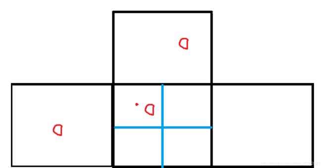
目标中心点为图中的红色点,红色点在本网格的左上,则让本网格、其左、其上网格负责该目标检测;
同理目标中心点如果在右下,则让本网格、其右、其下网格负责该目标检测。为什么这样做,据说是为了扩充正样本。
总结
核心代码差不多就是这些了