卡尔曼滤波器,这是一种使用噪声传感器测量(和贝叶斯规则)来生成未知量的可靠估计的算法(例如车辆可能在3秒内的位置)。
我们知道高斯方程包含两个主要参数:
- 一个是平均数
- 一个是方差,通常写为平方值。
一般来说,高斯方程是这样的:
我们将该方程的第一部分称为 系数,第二部分称为 指数。第二部分在定义高斯的形状时最为重要,而系数是一个归一化因子。
对于不确定的连续数量,例如自动驾驶汽车的预估位置,我们使用高斯方程来表示该数量的不确定性。方差越小,我们对数量越有把握。
# import math functions
from math import *
import matplotlib.pyplot as plt
import numpy as np

# gaussian function
def f(mu, sigma2, x):
    ''' f takes in a mean and squared variance, and an input x
       and returns the gaussian value.'''
    coefficient = 1.0 / sqrt(2.0 * pi *sigma2)
    exponential = exp(-0.5 * (x-mu) ** 2 / sigma2)
    return coefficient * exponential
# an example Gaussian
gauss_1 = f(10, 4, 8)
print(gauss_1)
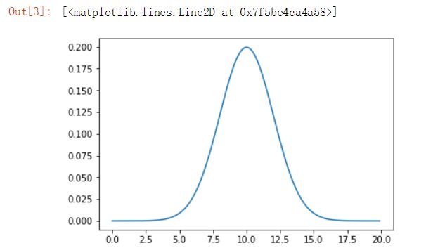
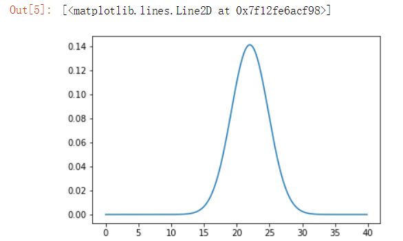
绘制高斯分布图
由于我们的函数仅返回x的特定值的值,因此我们可以通过遍历x值范围并创建高斯分布值g的结果列表来绘制高斯分布图
# display a gaussian over a range of x values
# define the parameters
mu = 10
sigma2 = 4

# define a range of x values
x_axis = np.arange(0, 20, 0.1)

# create a corresponding list of gaussian values
g = []
for x in x_axis:
    g.append(f(mu, sigma2, x))

# plot the result
plt.plot(x_axis, g)
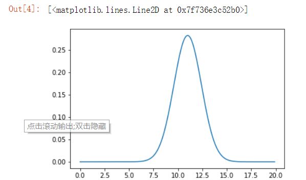
新的均值和方差

该程序要接收两个均值和方差,并为高斯方程返回一个全新的、已更新的均值和方差。此步骤称为参数或测量更新,因为它是当初始置信度(由下面的蓝色高斯表示)与新信息(具有一定不确定性的测量,即橙色高斯))合并时发生的更新。
已知两个均值和方差:
更新之后的公式:
更新的高斯将是这两个高斯的组合,其中新的均值介于两者之间,并且方差小于两个给定方差中的最小值。这意味着在测量之后,我们的新均值比初始置信度更加确定!
# import math functions
from math import *
import matplotlib.pyplot as plt
import numpy as np

# gaussian function
def f(mu, sigma2, x):
    ''' f takes in a mean and squared variance, and an input x
       and returns the gaussian value.'''
    coefficient = 1.0 / sqrt(2.0 * pi *sigma2)
    exponential = exp(-0.5 * (x-mu) ** 2 / sigma2)
    return coefficient * exponential
# the update function
def update(mean1, var1, mean2, var2):
    ''' This function takes in two means and two squared variance terms,
        and returns updated gaussian parameters.'''
    ## TODO: Calculate the new parameters
    new_mean = (var2 * mean1 + var1 * mean2) / (var1 + var2)
    new_var = 1 / (1 / var1 + 1 / var2)

    return [new_mean, new_var]
# display a gaussian over a range of x values
# define the parameters
mu = new_params[0]
sigma2 = new_params[1]

# define a range of x values
x_axis = np.arange(0, 20, 0.1)

# create a corresponding list of gaussian values
g = []
for x in x_axis:
    g.append(f(mu, sigma2, x))

# plot the result
plt.plot(x_axis, g)
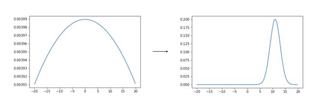
高斯函数移动
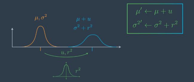
收集一些新测量之后,执行参数更新,然后,下一步是将运动合并到我们的高斯计算中。回想一下,在我们判断机器人或自动驾驶汽车位置的时候:
- 测量更新增加了 我们的判断确定性
- 运动更新/预测降低了我们的判断确定性
这是因为每次运动都有可能未达到或超越预期目的位置,并且由于运动的不准确性,我们最终会在每次运动后失去对确切位置的判断确定性。
# import math functions
from math import *
import matplotlib.pyplot as plt
import numpy as np

# gaussian function
def f(mu, sigma2, x):
    ''' f takes in a mean and squared variance, and an input x
       and returns the gaussian value.'''
    coefficient = 1.0 / sqrt(2.0 * pi *sigma2)
    exponential = exp(-0.5 * (x-mu) ** 2 / sigma2)
    return coefficient * exponential
# the update function
def update(mean1, var1, mean2, var2):
    ''' This function takes in two means and two squared variance terms,
        and returns updated gaussian parameters.'''
    # Calculate the new parameters
    new_mean = (var2*mean1 + var1*mean2)/(var2+var1)
    new_var = 1/(1/var2 + 1/var1)

    return [new_mean, new_var]
# the motion update/predict function
def predict(mean1, var1, mean2, var2):
    ''' This function takes in two means and two squared variance terms,
        and returns updated gaussian parameters, after motion.'''
    ## TODO: Calculate the new parameters
    new_mean = mean1 + mean2
    new_var = var1 + var2

    return [new_mean, new_var]
通过遍历一系列x值并创建高斯值 g的结果列表来绘制一个高斯图,如下所示。你可以尝试更改mu和sigma2的值,看一看会发生什么。
# display a gaussian over a range of x values
# define the parameters
mu = new_params[0]
sigma2 = new_params[1]

# define a range of x values
x_axis = np.arange(0, 40, 0.1)

# create a corresponding list of gaussian values
g = []
for x in x_axis:
    g.append(f(mu, sigma2, x))

# plot the result
plt.plot(x_axis, g)
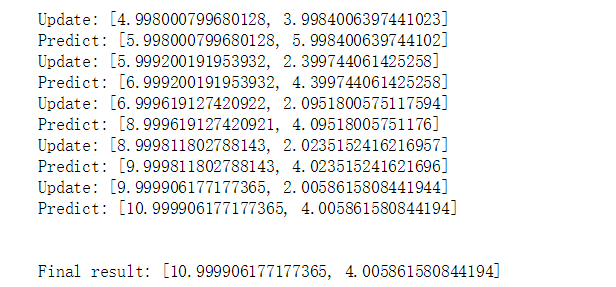
1D 卡尔曼滤波器代码
机器人在这个空间中移动时,它会通过执行以下循环来定位自己:
- 感测并执行测量更新任务
-
移动并执行动作更新任务
实现此滤波器后,你应该看到,一个非常不确定的位置高斯会变为一个越来越确定的高斯,如下图所示。
下面是常用的高斯方程和导入。
# import math functions
from math import *
import matplotlib.pyplot as plt
import numpy as np

# gaussian function
def f(mu, sigma2, x):
    ''' f takes in a mean and squared variance, and an input x
       and returns the gaussian value.'''
    coefficient = 1.0 / sqrt(2.0 * pi *sigma2)
    exponential = exp(-0.5 * (x-mu) ** 2 / sigma2)
    return coefficient * exponential
以下是update代码,该代码在合并初始置信度和新测量信息时执行参数更新。此外,完整的predict代码在合并一个运动后会对高斯值进行更新。
```python
# the update function
def update(mean1, var1, mean2, var2):
    ''' This function takes in two means and two squared variance terms,
        and returns updated gaussian parameters.'''
    # Calculate the new parameters
    new_mean = (var2*mean1 + var1*mean2)/(var2+var1)
    new_var = 1/(1/var2 + 1/var1)

    return [new_mean, new_var]
# the motion update/predict function
def predict(mean1, var1, mean2, var2):
    ''' This function takes in two means and two squared variance terms,
        and returns updated gaussian parameters, after motion.'''
    # Calculate the new parameters
    new_mean = mean1 + mean2
    new_var = var1 + var2

    return [new_mean, new_var]
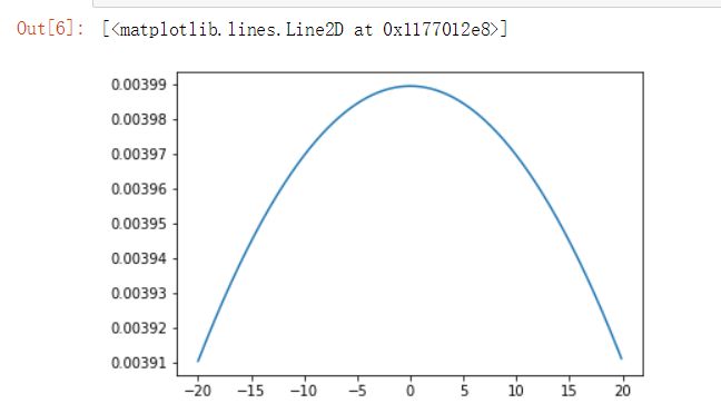
初始不确定性
初始参数,其中包括初始位置估计mu 和平方方差sig。注意,初始估计设置为位置0,方差非常大;这是一种高度混乱的状态,就像我们在直方图滤波器中使用的 均匀 分布一样。
# measurements for mu and motions, U
measurements = [5., 6., 7., 9., 10.]
motions = [1., 1., 2., 1., 1.]

# initial parameters
measurement_sig = 4.
motion_sig = 2.
mu = 0.
sig = 10000.

## TODO: Loop through all measurements/motions
## Print out and display the resulting Gaussian

# your code here
## TODO: Loop through all measurements/motions
# this code assumes measurements and motions have the same length
# so their updates can be performed in pairs
for n in range(len(measurements)):
    # measurement update, with uncertainty
    mu, sig = update(mu, sig, measurements[n], measurement_sig)
    print('Update: [{}, {}]'.format(mu, sig))
    # motion update, with uncertainty
    mu, sig = predict(mu, sig, motions[n], motion_sig)
    print('Predict: [{}, {}]'.format(mu, sig))


# print the final, resultant mu, sig
print('\n')
print('Final result: [{}, {}]'.format(mu, sig))
## Print out and display the final, resulting Gaussian
# set the parameters equal to the output of the Kalman filter result
mu = mu
sigma2 = sig

# define a range of x values
x_axis = np.arange(-20, 20, 0.1)

# create a corresponding list of gaussian values
g = []
for x in x_axis:
    g.append(f(mu, sigma2, x))

# plot the result
plt.plot(x_axis, g)