Python简单绘图一
其实一直都想学习一下Python,但是程序员都知道,只有当你真正用到一门语言的时候,学起来效率最高,所以我现在要用了
本来这个画图的工作,同事已经用MATLAB完成了,但是我自己一直觉得MATLAB不感冒,所以尝试用Python来做。
例子:http://matplotlib.org/examples/index.html
首先在Ubuntu16.04系统自带了Python(怎么方便怎么来)

需要安装pip

安装依赖库


OK 开始操练
1、画直线
import numpy as np
import matplotlib.pyplot as plt

x=[0,1]
y=[0,1]
plt.figure()
plt.plot(x,y)
plt.show()
#plt.savefig("easyplot.jpg")
2、画圆
from matplotlib.patches import Ellipse, Circle

import matplotlib.pyplot as plt
fig = plt.figure()
ax = fig.add_subplot(111)
cir1 = Circle(xy = (0.0, 1.0), radius=3, alpha=0.4)
ax.add_patch(cir1)
plt.axis('scaled')
plt.axis('equal')
plt.title('circle')
plt.show()
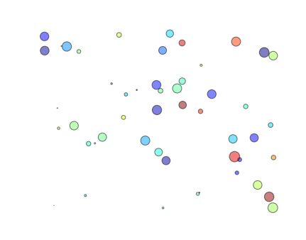
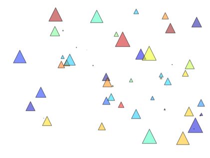
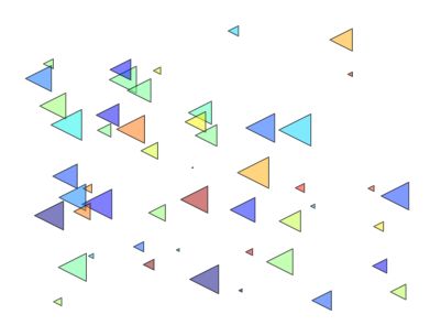
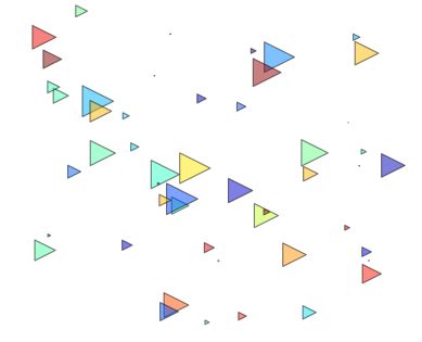
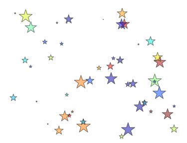
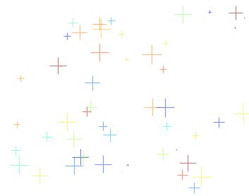
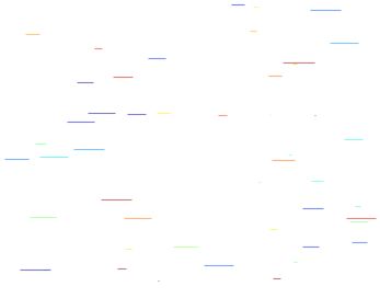
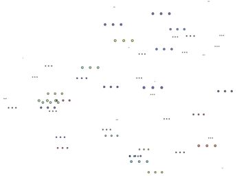
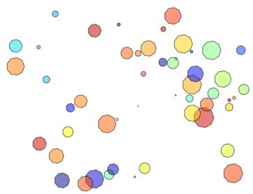
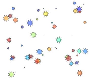
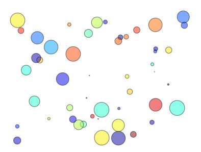
3、画散点图(这个就是我目前主要用到的)
from numpy import *;
import numpy as np
import matplotlib.pyplot as plt

N = 50
x = np.random.rand(N)
y = np.random.rand(N)
colors = np.random.rand(N)
area = np.pi * (15 * np.random.rand(N))**2
plt.scatter(x, y, s=area, c=colors, alpha=0.5, marker=(9, 3, 30))
plt.show()
这里用到一个matplotlib.pyplot子库中画散点图的函数
matplotlib.pyplot.scatter(x, y, s=20, c=None, marker='o',
 cmap=None, norm=None, vmin=None, vmax=None, alpha=None,
 linewidths=None, verts=None, edgecolors=None, hold=None,
 data=None, **kwargs)
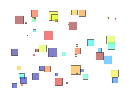
这个函数接收的参数很多,有默认值的平时也不需要我们指定,是可选的,这次我们用到的除了基本的x ,y参数,还有c,s,alpha和marker,c就是为点指定的颜色数组,s是点的面积大小,alpha是点的颜色的透明度,marker是指定点标记的形状。在例子里指定透明度为0.5,c和s是随机生成的,我们要改变的是marker的值,marker有很多值可供选择,下表展示了在例子代码的基础上,改变marker的值后的效果:
| marker | result |
|---|---|
| ”.” |  |
| ”,” |  |
| “o” | 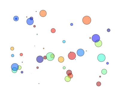 |
| “v” | 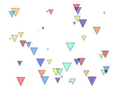 |
| “^” |  |
| “<” |  |
| “>” |  |
| “1” | 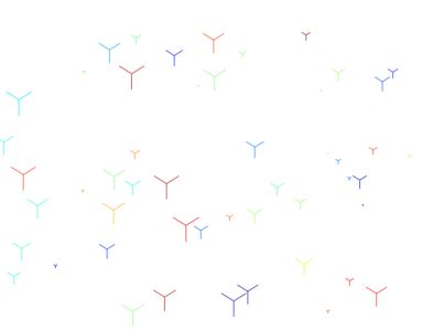 |
| “2” | 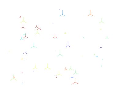 |
| “3” | 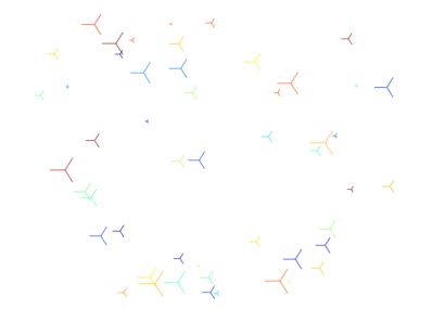 |
| “4” | 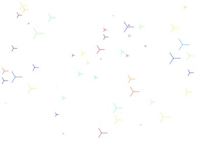 |
| “8” |  |
| “s” |  |
| “p” |  |
| “*” |  |
| “h” |  |
| “H” | 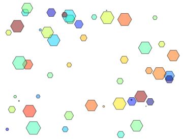 |
| “+” |  |
| “x” | 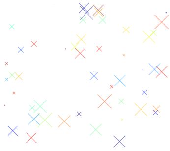 |
| “D” | 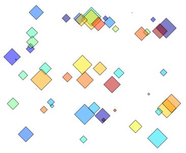 |
| “d” | 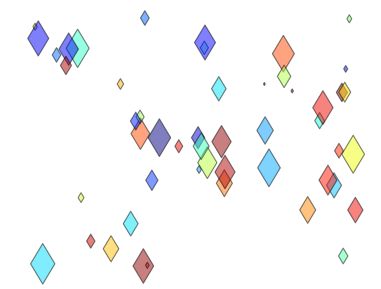 |
| “ | ” |
| “_” |  |
| “None” | 没错就是什么都没有。。。 |
| “$…$” |  |
| (numsides, style, angle) eg:(9,0, 30) 注:numsides是边的个数, angle是旋转角度, style只有0,1,2,3四个值 |
 |
| (numsides, style, angle) eg:(9,1, 30) |
 |
| (numsides, style, angle) eg:(9,2, 30) |
 |
| (numsides, style, angle) eg:(9,3, 30) 注:此时numsides和angle的值自动被忽略 |
 |
4、各种形状
import matplotlib.pyplot as plt
plt.rcdefaults()

import numpy as np
import matplotlib.pyplot as plt
import matplotlib.path as mpath
import matplotlib.lines as mlines
import matplotlib.patches as mpatches
from matplotlib.collections import PatchCollection


def label(xy, text):
    y = xy[1] - 0.15  # shift y-value for label so that it's below the artist
    plt.text(xy[0], y, text, ha="center", family='sans-serif', size=14)


fig, ax = plt.subplots()
# create 3x3 grid to plot the artists
grid = np.mgrid[0.2:0.8:3j, 0.2:0.8:3j].reshape(2, -1).T

patches = []

# add a circle
circle = mpatches.Circle(grid[0], 0.1, ec="none")
patches.append(circle)
label(grid[0], "Circle")

# add a rectangle
rect = mpatches.Rectangle(grid[1] - [0.025, 0.05], 0.05, 0.1, ec="none")
patches.append(rect)
label(grid[1], "Rectangle")

# add a wedge
wedge = mpatches.Wedge(grid[2], 0.1, 30, 270, ec="none")
patches.append(wedge)
label(grid[2], "Wedge")

# add a Polygon
polygon = mpatches.RegularPolygon(grid[3], 5, 0.1)
patches.append(polygon)
label(grid[3], "Polygon")

# add an ellipse
ellipse = mpatches.Ellipse(grid[4], 0.2, 0.1)
patches.append(ellipse)
label(grid[4], "Ellipse")

# add an arrow
arrow = mpatches.Arrow(grid[5, 0] - 0.05, grid[5, 1] - 0.05, 0.1, 0.1, width=0.1)
patches.append(arrow)
label(grid[5], "Arrow")

# add a path patch
Path = mpath.Path
path_data = [
    (Path.MOVETO, [0.018, -0.11]),
    (Path.CURVE4, [-0.031, -0.051]),
    (Path.CURVE4, [-0.115,  0.073]),
    (Path.CURVE4, [-0.03 ,  0.073]),
    (Path.LINETO, [-0.011,  0.039]),
    (Path.CURVE4, [0.043,  0.121]),
    (Path.CURVE4, [0.075, -0.005]),
    (Path.CURVE4, [0.035, -0.027]),
    (Path.CLOSEPOLY, [0.018, -0.11])
    ]
codes, verts = zip(*path_data)
path = mpath.Path(verts + grid[6], codes)
patch = mpatches.PathPatch(path)
patches.append(patch)
label(grid[6], "PathPatch")

# add a fancy box
fancybox = mpatches.FancyBboxPatch(
    grid[7] - [0.025, 0.05], 0.05, 0.1,
    boxstyle=mpatches.BoxStyle("Round", pad=0.02))
patches.append(fancybox)
label(grid[7], "FancyBboxPatch")

# add a line
x, y = np.array([[-0.06, 0.0, 0.1], [0.05, -0.05, 0.05]])
line = mlines.Line2D(x + grid[8, 0], y + grid[8, 1], lw=5., alpha=0.3)
label(grid[8], "Line2D")

colors = np.linspace(0, 1, len(patches))
collection = PatchCollection(patches, cmap=plt.cm.hsv, alpha=0.3)
collection.set_array(np.array(colors))
ax.add_collection(collection)
ax.add_line(line)

plt.subplots_adjust(left=0, right=1, bottom=0, top=1)
plt.axis('equal')
plt.axis('off')

plt.show()